Reconstructing plasma resistance from a measured signal.#
This example shows how to extract the resistance of a plasma load from either:
measured voltage and measured current, at the same position,
measured voltage and knowledge of the generator voltage,
measured current and knowledge of the generator voltage.
First, we import the required libraries.#
We start by importing the modules we need:
matplotlib for drawing graphs,
numpy for array functions,
pyresiflex for the generator, load and transmission solution.
import matplotlib.pyplot as plt
import numpy as np

from pyresiflex.cable.cable import PerfectCable
from pyresiflex.experiment.purely_resistive_experiment import (
    PurelyResistiveExperiment,
)
from pyresiflex.generator.generator_real_impedance import TrapezoidalGenerator
from pyresiflex.load.time_varying_resistance import PlasmaResistanceLinearFall
from pyresiflex.misc.plot import set_mpl_style
from pyresiflex.solver.purely_resistive_solution import PurelyResistiveSolution

set_mpl_style(nb_columns=2)
Transmission line parameters#
Generator parameters#
Load parameters#
Z_start = 1e3  # Start impedance [Ohm]
Z_end = 10  # End impedance [Ohm]
t_start_fall = L / c + 5e-9  # Start fall time [s]
t_end_fall = L / c + 10e-9  # End fall time [s]

plasma_load = PlasmaResistanceLinearFall(
    Z_start=Z_start,
    Z_end=Z_end,
    t_start_fall=t_start_fall,
    t_end_fall=t_end_fall,
)
Solution object.#
solution = PurelyResistiveSolution(
    generator=generator,
    load=plasma_load,
    cable=cable,
)
Generate voltage and current signals at a given position.#
# Define time vector.
times = np.arange(0, 200, 0.1) * 1e-9

x_meas_voltage = 2 / 3 * L
voltages = np.array([solution.V(x_meas_voltage, t) for t in times])

x_meas_current = 2 / 3 * L
currents = np.array([solution.I(x_meas_current, t) for t in times])
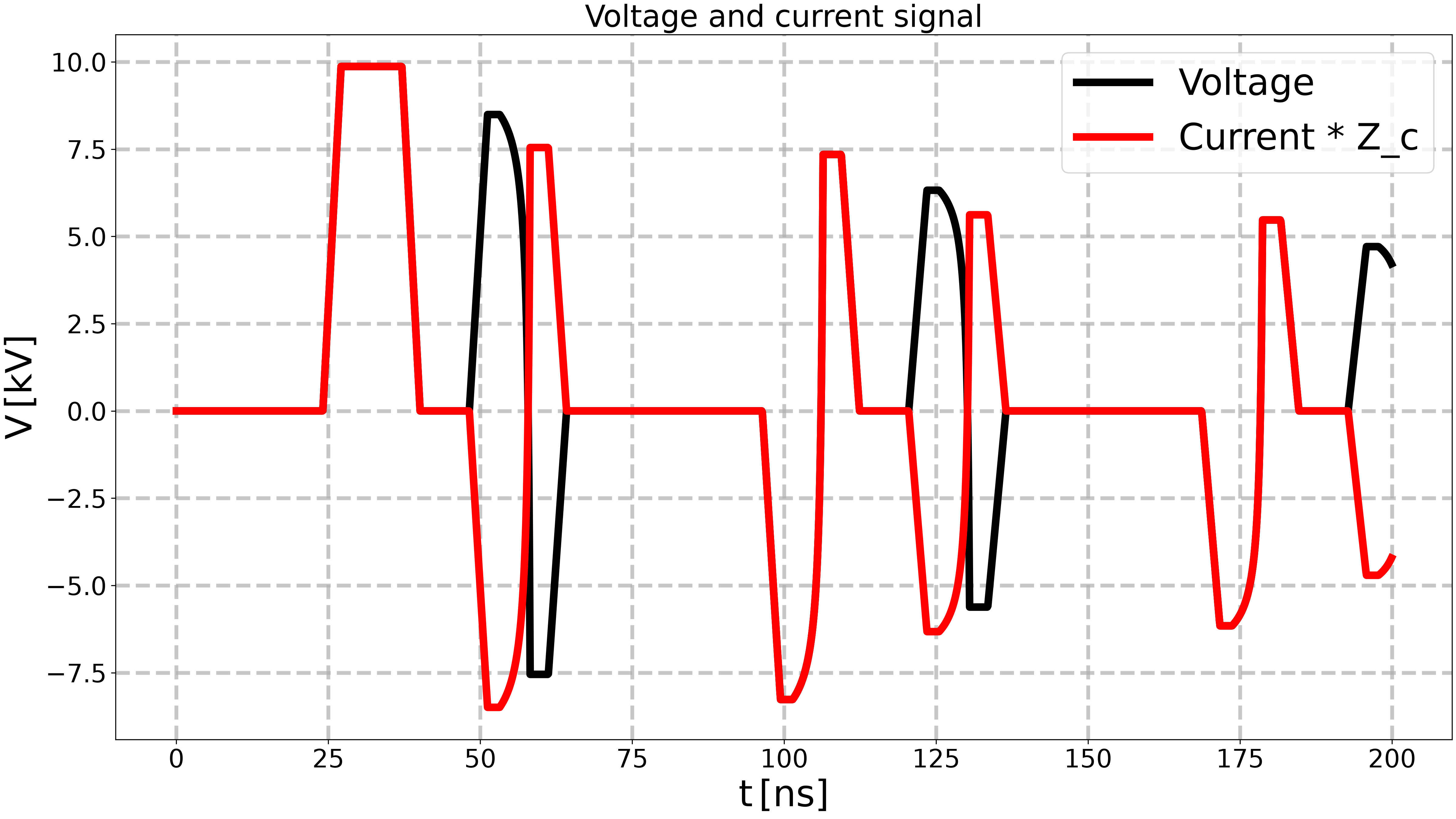
Plot the voltage and current signals.#
fig, ax = plt.subplots()

ax.plot(times * 1e9, voltages * 1e-3, color="k", label="Voltage")
ax.plot(times * 1e9, currents * Z_c * 1e-3, color="r", label="Current * Z_c")
ax.set_title("Voltage and current signal")
ax.set_xlabel(r"$\mathregular{t \, [ns]}$")
ax.set_ylabel(r"$\mathregular{V \, [kV]}$")
ax.legend()
plt.show()
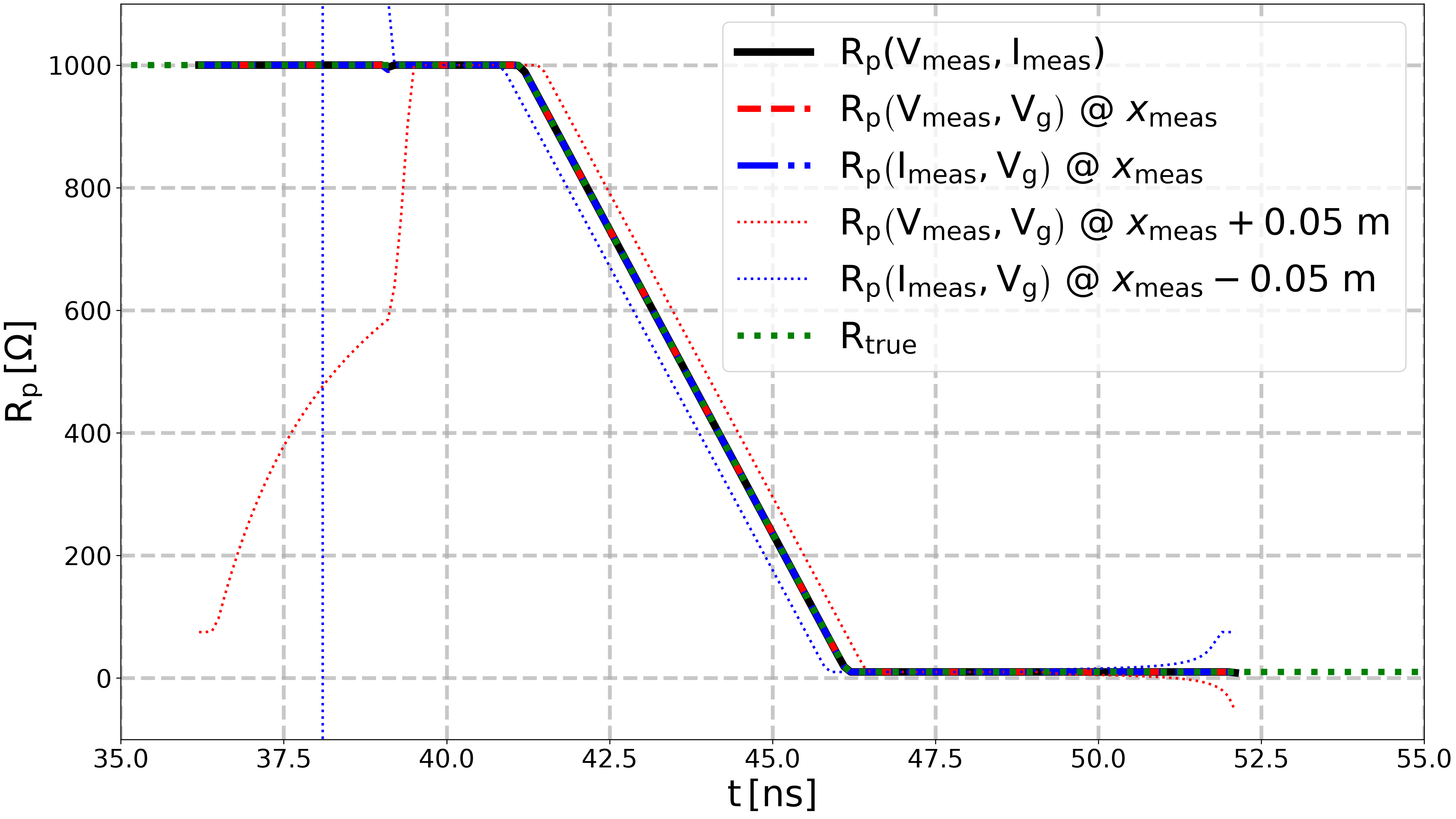
Compute the resistance from the voltage and current signals.#
This is possible since the voltage and current signals are measured at the same position.
expe = PurelyResistiveExperiment(
    experimental_voltage_time=times,
    experimental_voltage_value=voltages,
    x_meas_voltage=x_meas_voltage,
    experimental_current_time=times,
    experimental_current_value=currents,
    x_meas_current=x_meas_current,
    L=L,
    Z_c=Z_c,
    c=c,
    correct_time_zero=False,
)


# Compute R_p(vmeas, imeas)
expe.compute_plasma_resistance_from_vmeas_and_imeas(times)
# Compute R_p(vmeas, vg)
reconstructed_resistance_voltage = (
    expe.compute_plasma_resistance_from_vmeas_and_vg(
        times,
        generator=generator,
        max_n=4,
    )
)
# Compute R_p(imeas, vg)
reconstructed_resistance_current = (
    expe.compute_plasma_resistance_from_imeas_and_vg(
        times,
        generator=generator,
        max_n=4,
    )
)


expe_shifted = PurelyResistiveExperiment(
    experimental_voltage_time=times,
    experimental_voltage_value=voltages,
    x_meas_voltage=x_meas_voltage + 0.05,
    experimental_current_time=times,
    experimental_current_value=currents,
    x_meas_current=x_meas_current - 0.05,
    L=L,
    Z_c=Z_c,
    c=c,
    correct_time_zero=False,
)
# Compute R_p(vmeas, imeas)
# expe_shifted.compute_plasma_resistance_from_vmeas_and_imeas(times)
# Compute R_p(vmeas, vg)
reconstructed_resistance_voltage_shifted = (
    expe_shifted.compute_plasma_resistance_from_vmeas_and_vg(
        times,
        generator=generator,
        max_n=4,
    )
)
# Compute R_p(imeas, vg)
reconstructed_resistance_current_shifted = (
    expe_shifted.compute_plasma_resistance_from_imeas_and_vg(
        times,
        generator=generator,
        max_n=4,
    )
)
/home/runner/work/pyresiflex/pyresiflex/src/pyresiflex/experiment/purely_resistive_experiment.py:290: UserWarning: Some values in the denominator are zero, resistance cannot be computed correctly. These values are set to 1 MOhm.
  warn(
Compare the reconstructed resistance with the true resistance.#
set_mpl_style(nb_columns=2)

# Plot R_p(vmeas, imeas)
fig, ax = expe.plot_resistance(
    times=times,
    show=False,
    legend=False,
    plot_interpolated=False,
    _also_plot_when_near_cable_impedance=False,
)
# Change the line style and width of the existing plot.
for line in ax.get_lines():
    line.set_linestyle("-")


# Plot R_p(vmeas, vg)
ax.plot(
    times * 1e9, reconstructed_resistance_voltage, color="r", ls="--", lw=5
)
# Plot R_p(imeas, vg)
ax.plot(
    times * 1e9, reconstructed_resistance_current, color="b", ls="-.", lw=5
)

# Plot the shifted resistance.
# fig, ax = expe_shifted.plot_resistance(
#     times=times,
#     show=False,
#     legend=False,
#     plot_interpolated=False,
#     _also_plot_when_near_cable_impedance=False,
#     figax=(fig, ax),
# )
# ax.lines[-1].set_linestyle(":")
# ax.lines[-1].set_linewidth(2)
ax.plot(
    times * 1e9,
    reconstructed_resistance_voltage_shifted,
    color="r",
    ls=":",
    lw=2,
)
ax.plot(
    times * 1e9,
    reconstructed_resistance_current_shifted,
    color="b",
    ls=":",
    lw=2,
)


# Plot the true resistance.
true_resistance = np.array([plasma_load.load_impedance(t) for t in times])
ax.plot(times * 1e9, true_resistance, color="g", ls=":", lw=5)

# Plot options.
ax.set_ylim(-100, 1100)
ax.legend(
    [
        r"$\mathregular{R_p \left( V_{meas}, I_{meas} \right)}$",
        r"$\mathregular{R_p \left( V_{meas}, V_g \right)}$"
        + r" @ $x_{\text{meas}}$",
        r"$\mathregular{R_p \left( I_{meas}, V_g \right)}$"
        + r" @ $x_{\text{meas}}$",
        r"$\mathregular{R_p \left( V_{meas}, V_g \right)}$"
        + r" @ $x_{\text{meas}} + 0.05$ m",
        r"$\mathregular{R_p \left( I_{meas}, V_g \right)}$"
        + r" @ $x_{\text{meas}} - 0.05$ m",
        r"$\mathregular{R_{true}}$",
    ]
)

ax.set_xlim(35, 55)

plt.show()
Total running time of the script: (0 minutes 1.699 seconds)