Reproducing [Pavan2025] numerical simulations.

In this example, the load is a constant resistance in parallel with a constant capacitor.

Numerical data of [Pavan2025] are used for comparison between the analytical and numerical results. Voltage from Figure 8 of [Pavan2025] was digitized for this comparison.

This example also show how to create a custom load which inherits from ComplexImpedanceBaseLoad.

# This sets the first figure as the thumbnail for the example gallery.
# sphinx_gallery_thumbnail_number = 1
# This displays each image separately in the example gallery.
# sphinx_gallery_multi_image = "single"

First, we import the required libraries.

We start by importing the modules we need:

• matplotlib for drawing graphs,

• numpy for array functions,

• pyresiflex for the generator, load and transmission line.

import matplotlib.pyplot as plt
import numpy as np

from pyresiflex.cable.cable import PerfectCable
from pyresiflex.generator.generator_complex_impedance import GaussianGenerator
from pyresiflex.load.base_load import ComplexImpedanceBaseLoad
from pyresiflex.misc.plot import set_mpl_style
from pyresiflex.misc.units import c_0
from pyresiflex.misc.utils import get_path_to_data
from pyresiflex.solver.steady_impedance_solution import SteadyImpedanceSolution

set_mpl_style(nb_columns=2)

Create a generator class.

In the case of [Pavan2025], the generator voltage is a Gaussian pulse, with no internal resistance and no internal capacitance.

• height: 5e3 [V]

• mean: 35e-9 [s]

• FWHM: 20e-9 [s]

• R_g: 0.0 [Ohm]

• C_g: 0.0 [F]

pavan_generator = GaussianGenerator(
    height=5e3,  # [V]
    mean=35e-9,  # [s]
    FWHM=20e-9,  # [s]
    R_g=0.0,  # [Ohm]
    C_g=0.0,  # [F]
)

Transmission line parameters.

The transmission line is modeled as a perfect cable. The data used here are the ones from [Pavan2025].

L = 10.0  # Length of the transmission line [m]
c = 0.67 * c_0  # Wave celerity [m/s]
Z_c = 50  # Characteristic impedance [Ohm]

pavan_cable = PerfectCable(
    L=L,
    Z_c=Z_c,
    c=c,
)

Create a load class.

[Pavan2025] uses a resistive load in parallel with a capacitive load. Since this kind of load is not defined in the pyresiflex library, we create a custom load class.

class PavanLoad(ComplexImpedanceBaseLoad):
    def __init__(self, R_l: float, C_l: float):
        """Create a load class for the Pavan2025 case.

        Parameters
        ----------
        R_l : float
            Load resistance [Ohm]
        C_l : float
            Load capacitance [F]
        """
        super().__init__(purely_resistive=False)
        self.R_l = R_l
        self.C_l = C_l

    def load_impedance(self, frequency: np.ndarray) -> np.ndarray:
        r"""Return the load impedance.

        In the case of [Pavan2025]_, the load impedance is a capacitor
        in parallel with a resistor.

        Parameters
        ----------
        frequency : np.ndarray
            Frequency array, in Hz.

        Return
        ------
        np.ndarray
            The load impedance, in Ohms.

        Notes
        -----
        For parallel impedances, the total impedance is given by:

        .. math::

            Z_{load} = \frac{1}{\frac{1}{Z_R} + \frac{1}{Z_C}}

        where:

        - :math:`Z_R = R_l` is the load resistance.
        - :math:`Z_C = \frac{1}{j \omega C_l}` is the load capacitance.
        """
        return self.R_l / (
            1 + 1j * 2 * np.pi * frequency * self.R_l * self.C_l
        )


# Characteristic capacitance, as used by [Pavan2025]_.
C_ch = 667 * 1e-12  # [F]

# Dictionary of load cases, with label and color.
pavan_loads: dict[str, dict[str, PavanLoad | str]] = {
    "Case A": {
        "load": PavanLoad(R_l=10 * Z_c, C_l=0.1 * C_ch),
        "color": "black",
    },
    "Case B": {
        "load": PavanLoad(R_l=10 * Z_c, C_l=0.01 * C_ch),
        "color": "red",
    },
    "Case C": {
        "load": PavanLoad(R_l=0.5 * Z_c, C_l=0.1 * C_ch),
        "color": "blue",
    },
    "Case D": {
        "load": PavanLoad(R_l=0.5 * Z_c, C_l=0.01 * C_ch),
        "color": "green",
    },
}

# Add [Pavan2025]_ adimensional voltage of Figure 8, for the four cases.
pavan_voltage = {}
for label in pavan_loads:
    pavan_voltage[label] = np.loadtxt(
        get_path_to_data("Pavan2025", "Fig8", f"voltage_Load_{label[-1]}.csv"),
        skiprows=3,
        delimiter=",",
        unpack=True,
    )
# Add [Pavan2025]_ adimensional current of Figure 8, for the four cases.
pavan_current = {}
for label in pavan_loads:
    pavan_current[label] = np.loadtxt(
        get_path_to_data("Pavan2025", "Fig8", f"current_Load_{label[-1]}.csv"),
        skiprows=3,
        delimiter=",",
        unpack=True,
    )
# Add [Pavan2025]_ adimensional energy of Figure 8, for the four cases.
pavan_energy = {}
for label in pavan_loads:
    pavan_energy[label] = np.loadtxt(
        get_path_to_data("Pavan2025", "Fig8", f"energy_Load_{label[-1]}.csv"),
        skiprows=3,
        delimiter=",",
        unpack=True,
    )

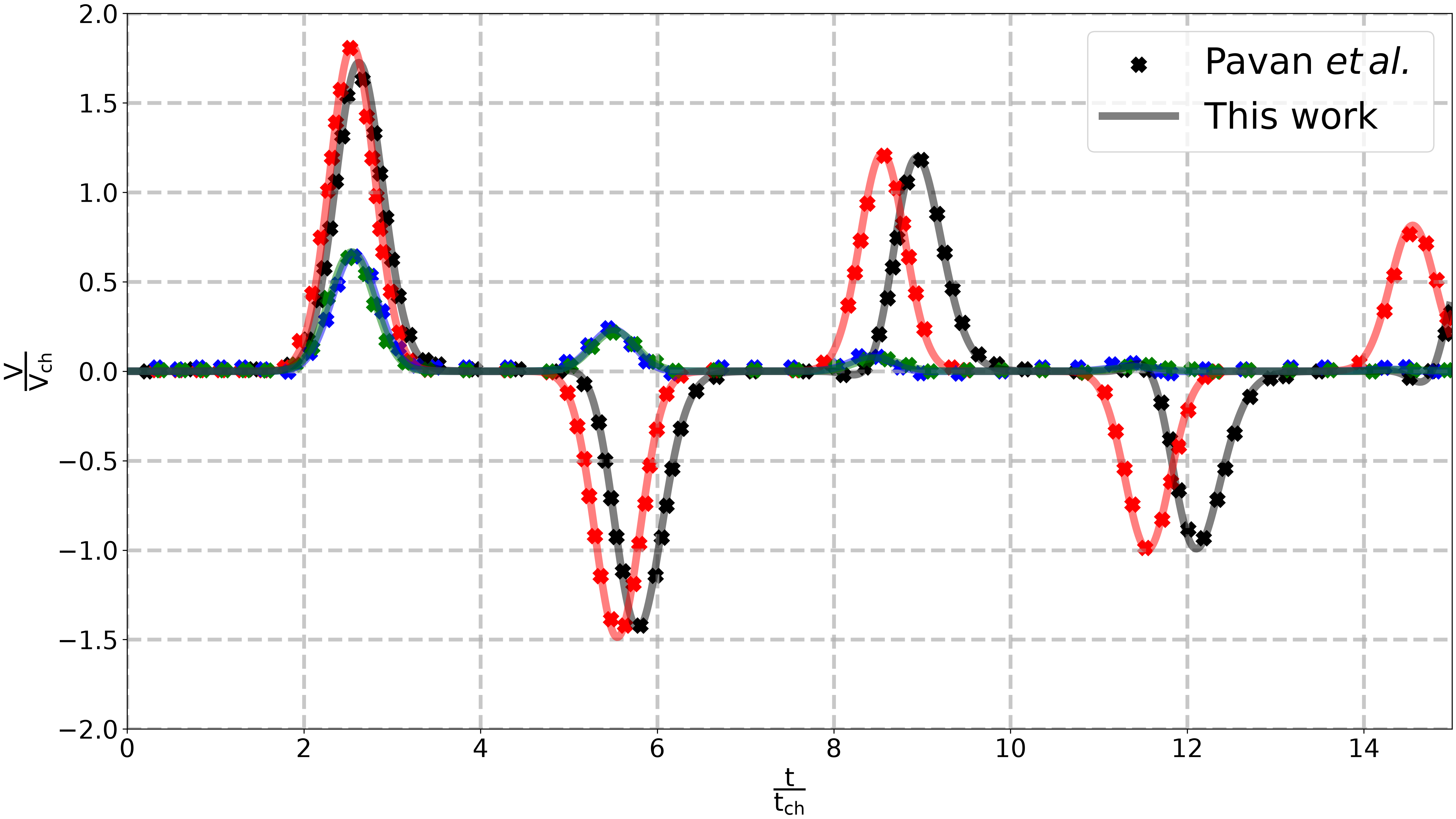
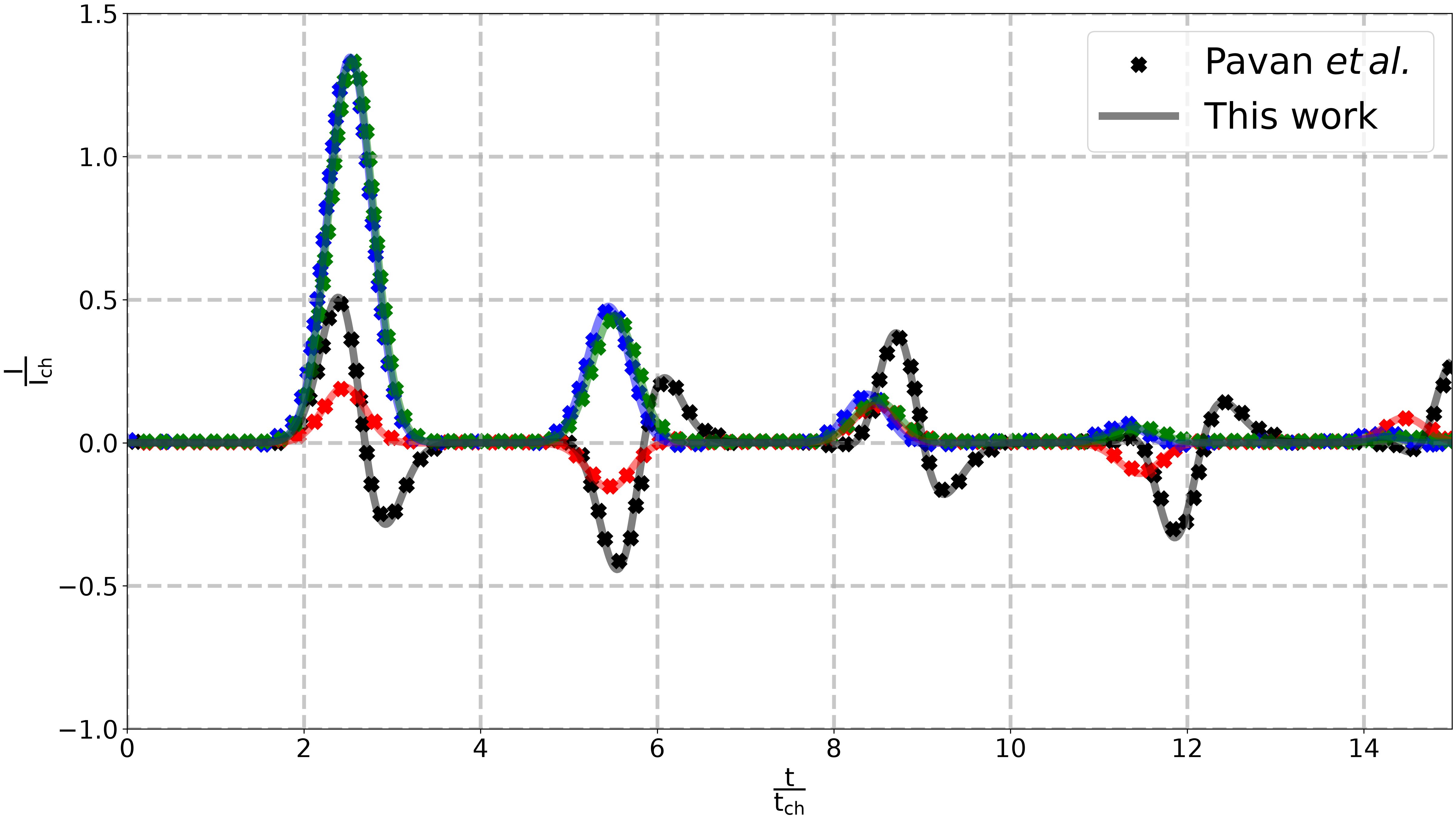
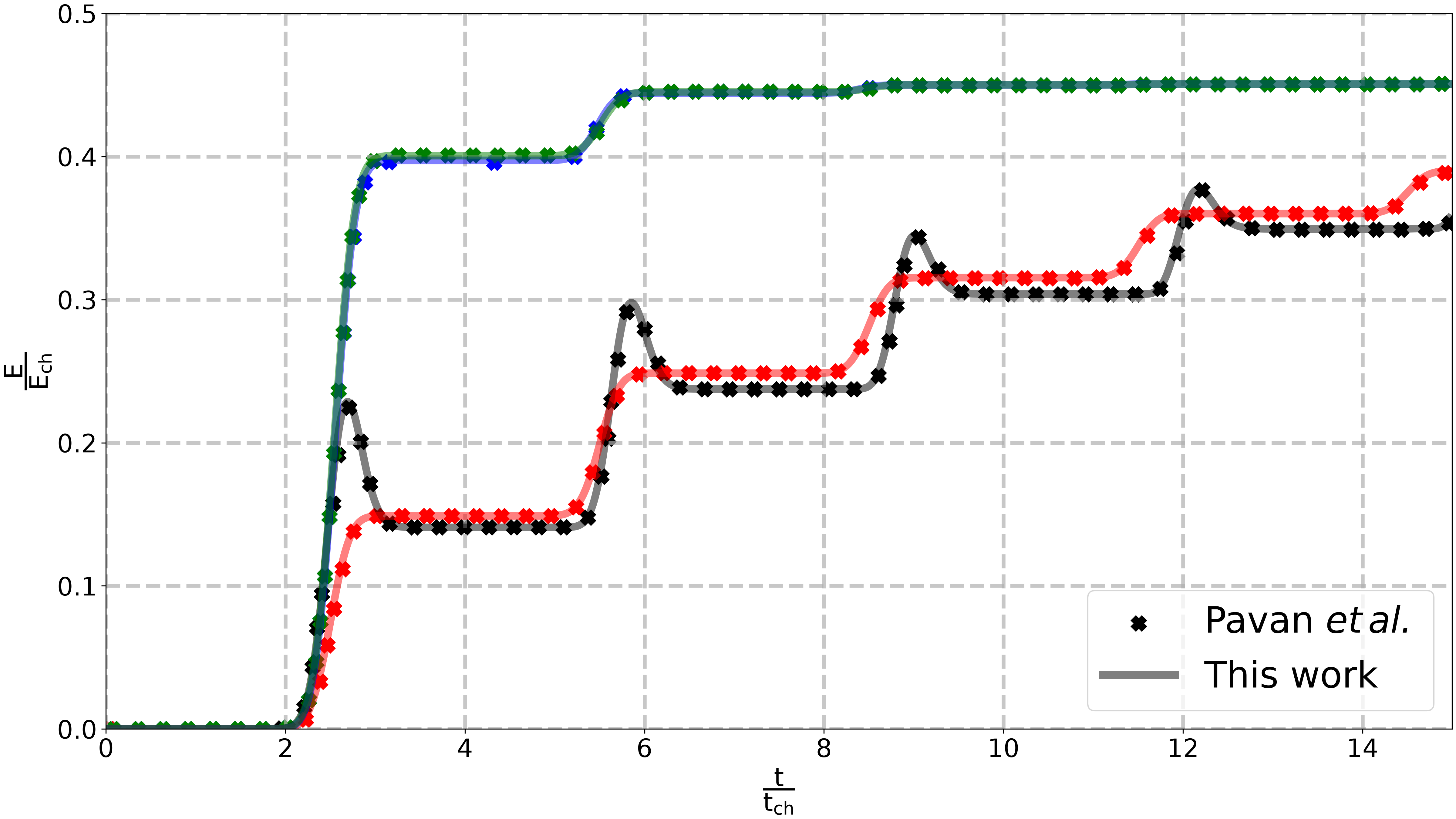
Solve and plot the results (Fig. 8 of [Pavan2025]).

This code reproduces the results from Figure 8 of [Pavan2025].

# Time array for the simulation.
times = np.linspace(0, 500, 1000, dtype=float) * 1e-9  # [s]
# Position of the voltage and current probes.
x = L  # [m]

# Characteristic values defined by [Pavan2025]_.
t_ch = 33.4 * 1e-9  # Characteristic time [s]
V_ch = 5e3  # Characteristic voltage [V]
I_ch = 100  # Characteristic current [A]
E_ch = 16.7e-3  # Characteristic energy [J]

# Parameters for Fourier Transform.
# Not given in [Pavan2025]_ so chosen arbitrarily to reproduce results.
# .. Number of points for Fourier transform.
nb_point_ft = 5_000  # Increase for better results (but higher cost).
# .. Maximum time for Fourier transform.
max_time_ft = 5_000e-9  # [s]  # Increase for better results (but higher cost).

# The generator, cable and Fourier-transform settings are shared by the four
# loads, so build each solution once here and reuse it for both Fig. 8 (probe
# at x = L) and Fig. 9 (probe at x = L / 2) below; only the load and the probe
# position passed to ``solve`` change.
solutions: dict[str, SteadyImpedanceSolution] = {}
for label, pavan_dict in pavan_loads.items():
    pavan_load = pavan_dict["load"]
    assert isinstance(pavan_load, ComplexImpedanceBaseLoad)
    solutions[label] = SteadyImpedanceSolution(
        generator=pavan_generator,
        load=pavan_load,
        cable=pavan_cable,
        nb_points_ft=nb_point_ft,
        max_time_ft=max_time_ft,
    )

fig_v, ax_v = plt.subplots()
fig_i, ax_i = plt.subplots()
fig_e, ax_e = plt.subplots()

marker_size = 80
marker_symbol = "x"
alpha = 0.5

for label, pavan_dict in pavan_loads.items():
    # Extract the colour from the dictionary.
    color = pavan_dict["color"]
    assert isinstance(color, str)

    # Reuse the pre-built solution; only the probe position changes.
    solution = solutions[label]
    solution.solve(x, t=times)

    # Plot the results.
    # .. Voltage
    ax_v.set_xlabel(r"$\mathregular{\frac{t}{t_{ch}}}$")
    ax_v.set_ylabel(r"$\mathregular{\frac{V}{V_{ch}}}$")
    ax_v.set_xlim(0, 15)
    ax_v.set_ylim(-2, 2)
    # Numerical result.
    t_ref, v_ref = pavan_voltage[label]
    ax_v.scatter(
        t_ref,
        v_ref,
        s=marker_size,
        color=color,
        marker=marker_symbol,
    )
    # Model result.
    ax_v.plot(
        times / t_ch,
        solution.voltage / V_ch,
        label=label,
        color=color,
        ls="-",
        alpha=alpha,
    )

    # .. Current
    ax_i.set_xlabel(r"$\mathregular{\frac{t}{t_{ch}}}$")
    ax_i.set_ylabel(r"$\mathregular{\frac{I}{I_{ch}}}$")
    ax_i.set_xlim(0, 15)
    ax_i.set_ylim(-1, 1.5)
    # Numerical result.
    t_ref, i_ref = pavan_current[label]
    ax_i.scatter(
        t_ref,
        i_ref,
        s=marker_size,
        color=color,
        marker=marker_symbol,
    )
    # Model result.
    ax_i.plot(
        times / t_ch,
        solution.current / I_ch,
        label=label,
        color=color,
        ls="-",
        alpha=alpha,
    )

    # .. Energy
    ax_e.set_xlabel(r"$\mathregular{\frac{t}{t_{ch}}}$")
    ax_e.set_ylabel(r"$\mathregular{\frac{E}{E_{ch}}}$")
    ax_e.set_xlim(0, 15)
    ax_e.set_ylim(0, 0.5)
    # Numerical result.
    t_ref, e_ref = pavan_energy[label]
    # Only select one point out of two for better visibility.
    t_ref = t_ref[::2]
    e_ref = e_ref[::2]
    ax_e.scatter(
        t_ref,
        e_ref,
        s=marker_size,
        color=color,
        marker=marker_symbol,
    )
    # Model result.
    ax_e.plot(
        times / t_ch,
        solution.energy / E_ch,
        label=label,
        color=color,
        ls="-",
        alpha=alpha,
    )

# Add legend for voltage figure.
line_v_numerical_legend = ax_v.scatter(
    [],
    [],
    color="black",
    s=marker_size,
    marker=marker_symbol,
)
(line_v_model_legend,) = ax_v.plot(
    [],
    [],
    color="black",
    ls="-",
    alpha=alpha,
)
ax_v.legend(
    [line_v_numerical_legend, line_v_model_legend],
    [r"Pavan $\it{et \, al.}$", "This work"],
    labelcolor="black",
    loc="upper right",
)
# Add legend for current figure.
line_i_numerical_legend = ax_i.scatter(
    [],
    [],
    color="black",
    s=marker_size,
    marker=marker_symbol,
)
(line_i_model_legend,) = ax_i.plot(
    [],
    [],
    color="black",
    ls="-",
    alpha=alpha,
)
ax_i.legend(
    [line_i_numerical_legend, line_i_model_legend],
    [r"Pavan $\it{et \, al.}$", "This work"],
    labelcolor="black",
    loc="upper right",
)
# Add legend for energy figure.
line_e_numerical_legend = ax_e.scatter(
    [],
    [],
    color="black",
    s=marker_size,
    marker=marker_symbol,
)
(line_e_model_legend,) = ax_e.plot(
    [],
    [],
    color="black",
    ls="-",
    alpha=alpha,
)
ax_e.legend(
    [line_e_numerical_legend, line_e_model_legend],
    [r"Pavan $\it{et \, al.}$", "This work"],
    labelcolor="black",
    loc="lower right",
)

plt.show()

# Save figures.
fig_v.savefig(
    get_path_to_data(
        "article_figures",
        "Pavan2024_comparison_fig8_voltage_at_load.svg",
        force_return=True,
    ),
)
fig_i.savefig(
    get_path_to_data(
        "article_figures",
        "Pavan2024_comparison_fig8_current_at_load.svg",
        force_return=True,
    ),
)
fig_e.savefig(
    get_path_to_data(
        "article_figures",
        "Pavan2024_comparison_fig8_energy_at_load.svg",
        force_return=True,
    ),
)

• 
• 
• 

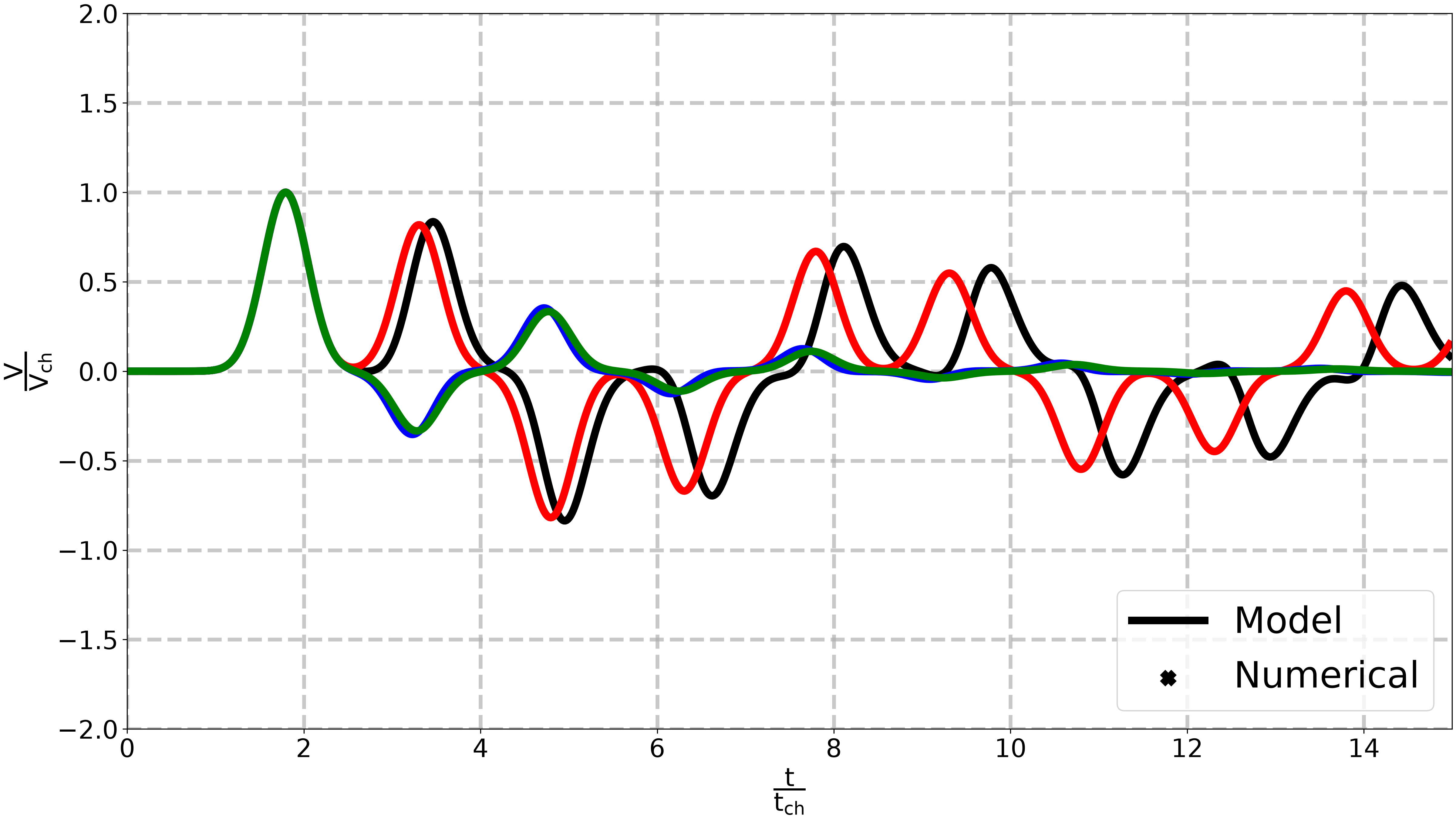
Solve and plot the results (Fig. 9 of [Pavan2025]).

This code reproduces the results from Figure 9 of [Pavan2025].

# The only change is the position of the measurement.
x = L / 2  # Position of the measurement in meters.
fig_v, ax_v = plt.subplots()
fig_i, ax_i = plt.subplots()
fig_e, ax_e = plt.subplots()


for label, pavan_dict in pavan_loads.items():
    # Extract the colour from the dictionary.
    color = pavan_dict["color"]
    assert isinstance(color, str)

    # Reuse the pre-built solution; only the probe position changes.
    solution = solutions[label]
    solution.solve(x, t=times)

    # Plot the results.
    # .. Voltage
    ax_v.plot(times / t_ch, solution.voltage / V_ch, label=label, color=color)
    ax_v.set_xlabel(r"$\mathregular{\frac{t}{t_{ch}}}$")
    ax_v.set_ylabel(r"$\mathregular{\frac{V}{V_{ch}}}$")
    ax_v.set_xlim(0, 15)
    ax_v.set_ylim(-2, 2)

    # .. Current
    ax_i.plot(times / t_ch, solution.current / I_ch, label=label, color=color)
    ax_i.set_xlabel(r"$\mathregular{\frac{t}{t_{ch}}}$")
    ax_i.set_ylabel(r"$\mathregular{\frac{I}{I_{ch}}}$")
    ax_i.legend()
    ax_i.set_xlim(0, 15)
    ax_i.set_ylim(-1, 1.5)

    # .. Energy
    ax_e.plot(times / t_ch, solution.energy / E_ch, label=label, color=color)
    ax_e.set_xlabel(r"$\mathregular{\frac{t}{t_{ch}}}$")
    ax_e.set_ylabel(r"$\mathregular{\frac{E}{E_{ch}}}$")
    ax_e.legend()
    ax_e.set_xlim(0, 15)
    ax_e.set_ylim(0, 0.5)

(line_v_model_legend,) = ax_v.plot([], [], color="black")
line_v_numerical_legend = ax_v.scatter(
    [],
    [],
    color="black",
    s=marker_size,
    marker=marker_symbol,
)
ax_v.legend(
    [line_v_model_legend, line_v_numerical_legend],
    ["Model", "Numerical"],
    labelcolor="black",
    loc="lower right",
)
plt.show()

• 
• 
•