Animation of an ideal pulse propagating in the cable.#
In this example, the plasma is modeled as a time-varying resistance.
To run the simulations, various parameters are needed:
for the transmission line:
Length \(L = 6.2 \, \mathrm{m}\)
Wave velocity \(c = 1.9 \times 10^8 \, \mathrm{m/s}\)
Characteristic impedance \(Z_\mathregular{c} = 75 \, \Omega\)
for the generator:
Generator voltage is a trapezoidal pulse with a plateau of \(7 \, \mathrm{kV}\) and a duration of 6 ns, a rise time of 5 ns and a fall time of 6 ns.
Internal resistance of \(R_\mathregular{g} = 1 \, \Omega\)
for the load:
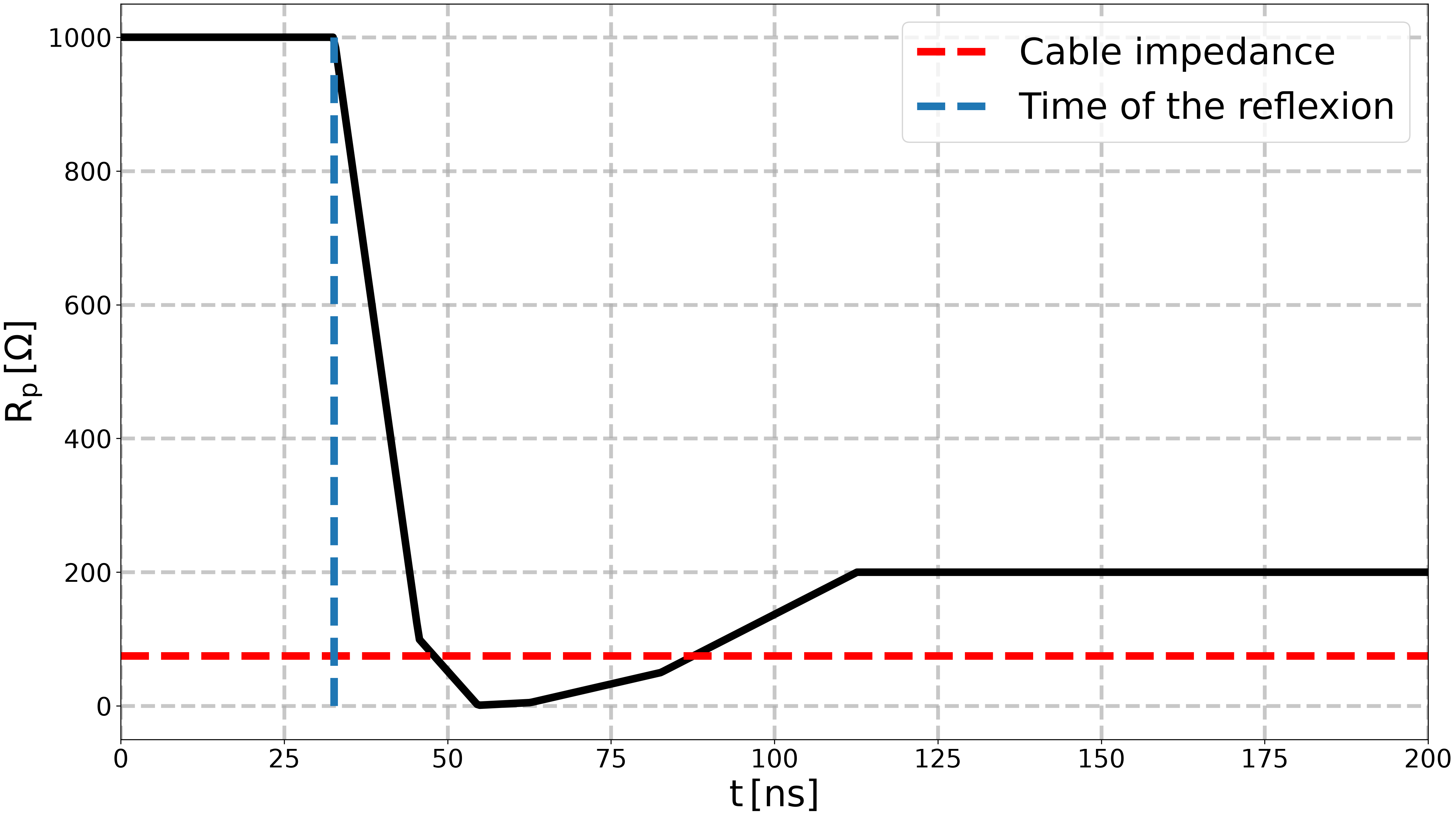
Plasma resistance is a time-varying resistance, whose values are manually chosen. First, high resistance (compared to the cable impedance). Then, it drops to a low value, before rising again.
First, we import the required libraries.#
We start by importing the modules we need:
matplotlib for drawing graphs,
numpy for array functions,
pyresiflex for the generator, load and transmission line.
import matplotlib.pyplot as plt
import numpy as np

from pyresiflex.cable.cable import PerfectCable
from pyresiflex.generator.generator_real_impedance import (
    TrapezoidalGenerator,
)
from pyresiflex.load.time_varying_resistance import PlasmaResistanceInterpolate
from pyresiflex.misc.plot import set_mpl_style
from pyresiflex.solver.purely_resistive_solution import PurelyResistiveSolution

set_mpl_style(nb_columns=2)
Time array.#
times = np.linspace(0, 200e-9, 500) # [s]
Transmission line parameters.#
# Transmission line parameters estimated from experimental data.
# See `plot_determine_Minesi2022_parameters.py` example for more details.

# Length of the transmission line
L = 6.2  # [m]
# Measurement points = probe positions
x = L / 2  # [m]
# Here, we assume that the probes are located at the same position.
x_meas_voltage = x_meas_current = x  # [m]
# Velocity of propagation of the wave in the cable.
c = 1.9e8  # [m/s]
# Cable characteristic impedance.
Z_c = 75  # [Ohm]

cable = PerfectCable(
    L=L,
    Z_c=Z_c,
    c=c,
)
Generator parameters.#
# Impedance of the generator.
R_g = 1  # [Ohm]

generator = TrapezoidalGenerator(
    R_g=R_g,
    U_off=0.0,
    U_on=7e3,
    t_rise=5e-9,
    t_on=6e-9,
    t_fall=6e-9,
)
Load parameters.#
plasma_load = PlasmaResistanceInterpolate(
    t_array=np.array([0, 13, 22, 30, 50, 80]) * 1e-9 + L / c,
    R_array=np.array([1000, 100, 1, 5, 50, 200]),
)

# Plot the plasma resistance vs time.
R_p = np.array([plasma_load.load_impedance(t) for t in times])

fig, ax = plt.subplots()
ax.plot(
    times * 1e9,
    R_p,
    color="k",
)
ax.set_xlabel(r"$\mathregular{t \, [ns]}$")
ax.set_ylabel(r"$\mathregular{R_p \, [\Omega]}$")
ax.hlines(
    Z_c,
    xmin=0,
    xmax=200,
    color="r",
    ls="--",
    label="Cable impedance",
)
ax.vlines(
    x=cable.L / cable.c * 1e9,
    ymin=0,
    ymax=1000,
    ls="--",
    label="Time of the reflexion",
)
ax.set_xlim(0, 200)
ax.legend()
plt.show()
Solution object.#
solution = PurelyResistiveSolution(
    generator=generator,
    load=plasma_load,
    cable=cable,
)
Compute voltage and current at a given position.#
# Time vector for the simulation.
nb_steps = 1000
# Position of probes for measurement
x = 3.1  # [m]


# Compute the voltage and current at probes' position.
solution.solve(x, times)

voltages = solution.voltage  # [V]
currents = solution.current  # [A]
energies = solution.energy  # [J]
xs = solution.x  # [m]
times = solution.t  # [s]
Plot the voltage and current at a given position.#
# This sets the following figure as the thumbnail for the example gallery.
# sphinx_gallery_thumbnail_number = 5

# Do we want to plot the current and energy?
plot_current = True
plot_energy = True


# Compute the min and max values of the voltage and current,
# to have the same zero level for voltage and current.
max_abs_voltage = np.max(np.abs(voltages)) * 1.1
max_abs_current = np.max(np.abs(currents)) * 1.1

fig, ax_v = plt.subplots()

# Plot voltage.
plot_line_v = ax_v.plot(
    (times - x / c) * 1e9,
    voltages * 1e-3,
    color="k",
    ls="-",
    label="Voltage (computed)",
)
# .. Plot options for voltage.
ax_v.set_xlabel(r"$\mathregular{t - \frac{x_{meas}}{c} \, [ns]}$")
ax_v.set_ylabel(r"$\mathregular{V \, [kV]}$")
ax_v.set_ylim(-8, 8)
ax_v.spines["left"].set_color("k")
ax_v.set_xlim(times[0] * 1e9, times[-1] * 1e9)

# Plot current.
if plot_current:
    ax_i = ax_v.twinx()
    plot_line_i = ax_i.plot(
        (times - x / c) * 1e9,
        currents,
        color="r",
        ls="-",
        label="Current (computed)",
    )
    # .. Plot options for current.
    ax_i.set_ylabel(r"$\mathregular{I \, [A]}$", color="r")
    # ax_i.set_ylim(-max_abs_current, max_abs_current)
    ax_i.set_ylim(-120, 120)
    ax_i.grid(visible=False)
    # Change color of the right y-axis to red.
    ax_i.spines["right"].set_color("r")
    # Also change the color of the ticks.
    ax_i.tick_params(axis="y", colors="r")
    # Move x-position of the y-label.
    ax_i.yaxis.set_label_coords(1.05, 0.5)

# Plot energy.
if plot_energy:
    ax_e = ax_v.twinx()
    plot_line_e = ax_e.plot(
        (times - x / c) * 1e9,
        energies * 1e3,
        color="b",
        ls="-",
        label="Energy",
    )
    # .. Plot options for energy.
    ax_e.set_ylabel(r"$\mathregular{E \, [mJ]}$", color="b")
    # Move the y-axis of ax_e to the right, by 100 points
    ax_e.spines["right"].set_position(("outward", 100))
    ax_e.grid(visible=False)
    ax_e.set_ylim(0, 8)
    # Change color of the right y-axis to blue.
    ax_e.spines["right"].set_color("b")
    # Also change the color of the ticks.
    ax_e.tick_params(axis="y", colors="b")


# .. Display all legends in the same box.
lines = plot_line_v
if plot_current and plot_line_i:
    lines += plot_line_i
if plot_energy and plot_line_e:
    lines += plot_line_e

labels: list[str] = []
for line in lines:
    label = line.get_label()
    if isinstance(label, str):
        labels.append(label)
    else:
        labels.append("Unknown")

ax_v.legend(
    handles=plot_line_v,
    labels=["Computed"],
    loc="lower right",
)

plt.show()
/home/runner/work/pyresiflex/pyresiflex/examples/pure_resistance_impedance/plot_animation_of_pulse.py:263: UserWarning: Mismatched number of handles and labels: len(handles) = 3 len(labels) = 1
  ax_v.legend(
Compute at different times for all positions and animate.#
# Define the space and time vectors.
N_x = 10  # Number of points in space (Increase it as needed).
xs = np.linspace(0, L, N_x, dtype=float)  # Space vector [m]

t_max = 200e-9  # Maximum time [s]
N_t = 10  # Number of points in time (Increase it as needed).
times = np.linspace(0, t_max, N_t, dtype=float)  # Time vector [s]

solution.solve(xs, times)

# Animate the voltage and current along the transmission line.
ani = solution.animation(
    interval=1000,
    with_current=False,
    y_min_max_voltage=(-8, 16),
)

# Save the animation as a .mp4 file.
# ani.save("animation_of_pulse_propagation.mp4", writer="ffmpeg", fps=10)

# # %%
# # Save the animation as a .gif file.
# import matplotlib.animation as animation  # noqa: E402

# writer = animation.PillowWriter(fps=15, bitrate=1800)
# ani.save("animation_of_pulse_propagation.gif", writer=writer)
Total running time of the script: (0 minutes 8.463 seconds)