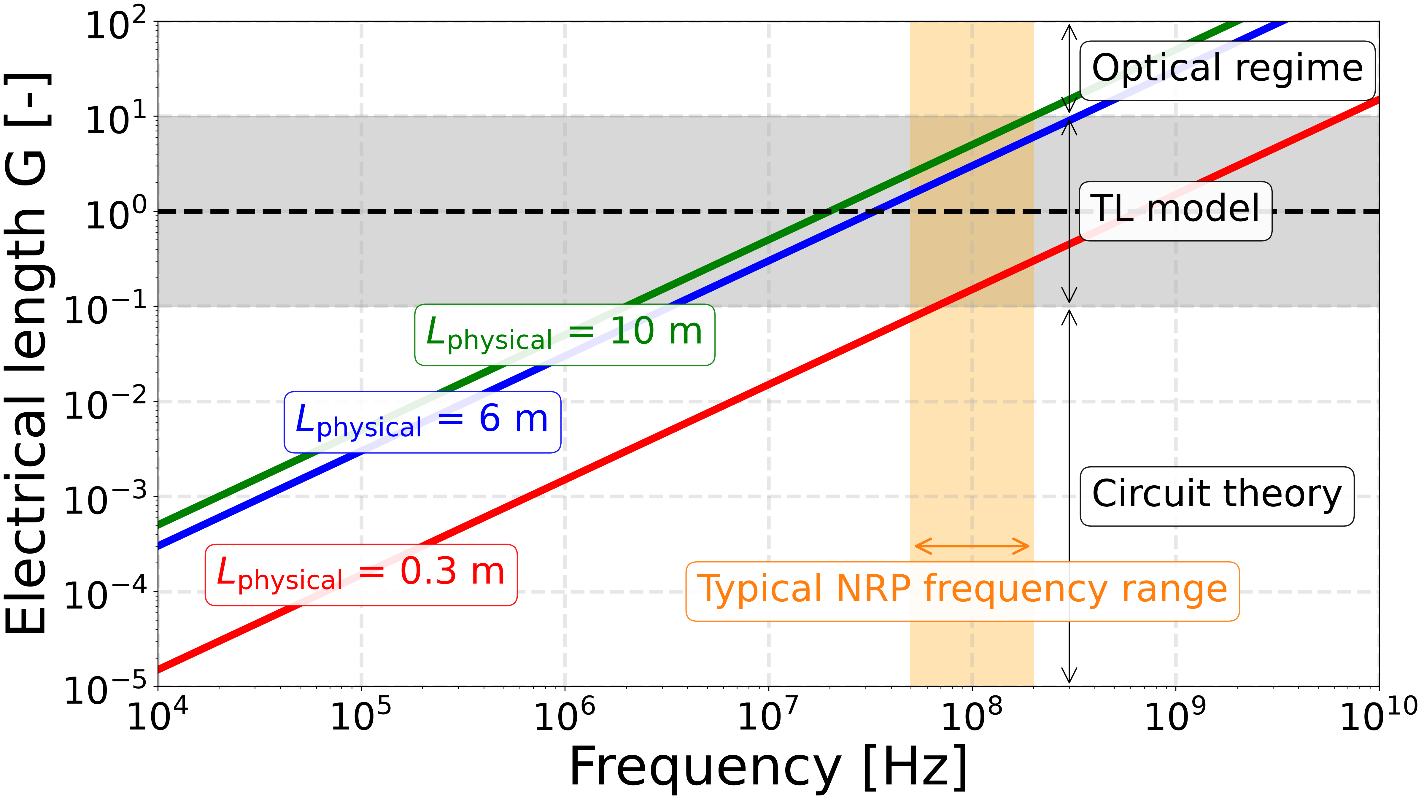
Electrical length of a coaxial cable and corresponding theory.

This example determines the electrical length of a coaxial cable as a function of frequency and physical length.

The definition used comes from [Wikipedia](https://en.wikipedia.org/wiki/Electrical_length#Definition):

\[G = \frac{L_\text{physical}}{\lambda} = \frac{f L_\text{physical}}{v_\text{p}}\]

where:

• \(G\) is the electrical length of the coaxial cable [dimensionless], corresponding to the number of wavelengths in the coaxial cable,

• \(L_\text{physical}\) is the physical length of the coaxial cable [m],

• \(\lambda\) is the wavelength of the signal in the coaxial cable [m],

• \(f\) is the frequency of the signal [Hz],

• \(v_\text{p}\) is the phase velocity of the signal in the coaxial cable [m/s], which is related to the speed of light in vacuum \(c_0\) by the phase velocity factor \(v_\text{p} = \text{phase velocity factor} \cdot c_0\).

Then, depending on the electrical length, different theories can be used to describe the behavior of the coaxial cable:

• For \(G < 0.1\), the circuit theory is valid, and Kirchhoff’s laws can be applied to the coaxial cable.

• For \(0.1 < G < 10\), the transmission line theory is valid, and the coaxial cable can be modeled as a transmission line.

• For \(G > 10\), the optical regime is valid, and the coaxial cable should be treated as an optical waveguide.

First, we import the required libraries.

We start by importing the modules we need:

• matplotlib for drawing graphs,

• numpy for array functions,

• pyresiflex for plot options and data loading.

import matplotlib.pyplot as plt
import numpy as np

import pyresiflex.misc.units as u
from pyresiflex.misc.plot import set_mpl_style
from pyresiflex.misc.utils import get_path_to_data

set_mpl_style(nb_columns=1)

Set parameters.

frequencies = np.geomspace(1e4, 1e10, 1000)  # [Hz]
phase_velocity_factor = 2 / 3  # [% of light speed]
physical_lengths = [0.3, 6, 10]  # [m]
xpos_label = [1e5, 2e5, 1e6]  # [Hz]
colors = ["red", "blue", "green"]


# Compute and plot the electrical length.
# ---------------------------------------

fig, ax = plt.subplots()

phase_velocity = phase_velocity_factor * u.c_0  # [m/s]

for physical_length, xpos, color in zip(physical_lengths, xpos_label, colors):
    wavelengths = phase_velocity / frequencies  # [m]
    electrical_length = physical_length / wavelengths  # [dimensionless]

    ax.loglog(
        frequencies,
        electrical_length,
        color=color,
    )
    ax.text(
        x=xpos,
        y=electrical_length[np.argmin(np.abs(frequencies - xpos))],
        s=r"$L_\text{physical}$ = " + f"{physical_length} m",
        verticalalignment="center",
        horizontalalignment="center",
        color=color,
        bbox=dict(
            facecolor="white",
            alpha=0.9,
            edgecolor=color,
            boxstyle="round",
        ),
    )

# Add vertical lines for electrical length = 1
ax.axhline(1, color="black", linestyle="--", lw=4)
ax.fill_between(frequencies, 0.1, 10, color="gray", alpha=0.3)

# Add horizontal lines for frequency used in NRP discharges.
f_min = 50e6  # [Hz]
f_max = 200e6  # [Hz]
ax.fill_betweenx([-1e5, 1e2], f_min, f_max, color="orange", alpha=0.3)
ax.annotate(
    "",
    xy=(f_min, 3e-4),
    xytext=(f_max, 3e-4),
    arrowprops=dict(arrowstyle="<->", color="tab:orange", lw=2),
)
ax.text(
    x=9e7,
    y=1e-4,
    s="Typical NRP frequency range",
    color="tab:orange",
    verticalalignment="center",
    horizontalalignment="center",
    bbox=dict(
        facecolor="white", alpha=0.9, boxstyle="round", edgecolor="tab:orange"
    ),
    zorder=10,
)


# Add 3 brackets, based on the electrical length, to show the different
# regimes of the coaxial cable.
# 1. Electrical length < 0.1; Circuit theory is valid.
ax.annotate(
    "",
    xy=(3e8, 1e-5),
    xytext=(3e8, 0.1),
    arrowprops=dict(arrowstyle="<->", color="black"),
)
ax.text(
    x=1.6e9,
    y=1e-3,
    s="Circuit theory",
    verticalalignment="center",
    horizontalalignment="center",
    bbox=dict(
        facecolor="white",
        alpha=0.9,
        boxstyle="round",
    ),
)
# 2. Electrical length between 0.1 and 10; Transmission line theory is valid.
ax.annotate(
    "",
    xy=(3e8, 0.1),
    xytext=(3e8, 10),
    arrowprops=dict(arrowstyle="<->", color="black"),
)
ax.text(
    x=1e9,
    y=1,
    s="TL model",
    verticalalignment="center",
    horizontalalignment="center",
    bbox=dict(
        facecolor="white",
        alpha=0.9,
        boxstyle="round",
    ),
)
# 3. Electrical length > 10; Optical regime is valid.
ax.annotate(
    "",
    xy=(3e8, 10),
    xytext=(3e8, 1e2),
    arrowprops=dict(arrowstyle="<->", color="black"),
)
ax.text(
    x=1.8e9,
    y=30,
    s="Optical regime",
    verticalalignment="center",
    horizontalalignment="center",
    bbox=dict(
        facecolor="white",
        alpha=0.9,
        boxstyle="round",
    ),
)


# Plot formatting
ax.set_xlabel("Frequency [Hz]")
ax.set_ylabel("Electrical length G [-]")
ax.set_xlim(np.min(frequencies), np.max(frequencies))
ax.set_ylim(1e-5, 1e2)
ax.grid(True, which="major", ls="--", alpha=0.3)
ax.grid(True, which="minor", ls="--", alpha=0.0)
plt.show()

Save the figure.

# Export the image to a .svg file, in the figures folder.
fig.savefig(
    get_path_to_data(
        "article_figures",
        "electrical_length.svg",
        force_return=True,
    ),
)