Considering parasitic capacitances/inductances in the system.

Before a plasma breakdown, the impedance of the gas can be represented as a very high resistance (no ionization) in parallel to a constant capacitance (representing the electrode and the surrounding environment).

The electrodes are generally placed in a reactor, which can have a small parasitic resistance and inductance, corresponding to the wires and the connections.

The equivalent circuit of the system is the following

  ----- R_wire --- L_wire -----┐-----┐
   ↑                           │     │   ↑
   │                           │     │   │
V(x=L, t)                     C_el  R_p  │ u_p(t)
   │                           │     │   │
   │       i_reactor           │     │   │
  ----------<------------------┘-----┘

Let us observe what are the current and voltage in this case.

# This sets the following figure as the thumbnail for the example gallery.
# sphinx_gallery_thumbnail_number = 5

First, we import the required libraries.

We start by importing the modules we need:

• matplotlib for drawing graphs,

• numpy for array functions,

• pyresiflex for the generator, load and transmission line.

import matplotlib.pyplot as plt
import numpy as np

from pyresiflex.cable.cable import PerfectCable
from pyresiflex.generator.generator_complex_impedance import GaussianGenerator
from pyresiflex.load.base_load import ComplexImpedanceBaseLoad
from pyresiflex.misc.units import c_0
from pyresiflex.misc.utils import get_path_to_data
from pyresiflex.solver.steady_impedance_solution import SteadyImpedanceSolution

plt.style.use(get_path_to_data("article_two_columns_figure.mplstyle"))

Create a trapezoidal generator.

generator = GaussianGenerator(
    height=4e3,  # [V]
    mean=5e-9,  # [s]
    FWHM=10e-9,  # [s]
    R_g=1.0,  # [Ohm]
    C_g=0,  # [F]
)

Transmission line parameters.

L = 4  # Length of the transmission line [m]
c = 0.67 * c_0  # Wave velocity [m/s]
Z_c = 75  # Characteristic impedance [Ohm]

cable = PerfectCable(
    L=L,
    Z_c=Z_c,
    c=c,
)

Create a load class for no breakdown plasma.

class ReactorImpedance(ComplexImpedanceBaseLoad):
    def __init__(self, R_wire, L_wire, C_electrode, R_plasma):
        super().__init__(purely_resistive=False)
        self.R_wire = R_wire
        self.L_wire = L_wire
        self.C_electrode = C_electrode
        self.R_plasma = R_plasma

    def load_impedance(self, frequency):
        # Load impedance is a capacitor in parallel with a resistor.
        Z_wire = self.R_wire + 1j * 2 * np.pi * frequency * self.L_wire

        # Combine the electrode capacitance and plasma resistance in parallel.
        # Z_electrode = 1 / (1j * 2 * np.pi * frequency * self.C_electrode)
        # Z_plasma = self.R_plasma
        # Z_el_plasma = 1 / (1 / Z_electrode + 1 / Z_plasma)
        Z_el_plasma = self.R_plasma / (
            1 + 1j * 2 * np.pi * frequency * self.C_electrode * self.R_plasma
        )
        return Z_wire + Z_el_plasma


no_breakdown_plasma = ReactorImpedance(
    R_wire=1e-3,  # Wire resistance [Ohm]
    L_wire=100e-9,  # Wire inductance [H]
    C_electrode=50e-12,  # Electrode capacitance [F]
    R_plasma=1e6,  # Plasma resistance [Ohm]
)

Solve the system.

# Create the solution object with the generator, load and cable.
solution = SteadyImpedanceSolution(
    generator=generator,
    load=no_breakdown_plasma,
    cable=cable,
    nb_points_ft=50_000,  # Number of points for Fourier transform.
    max_time_ft=50_000e-9,  # Maximum time for Fourier transform [s]
)

x_meas_voltage = L / 2  # Position of the measurement in meters.
x_meas_current = L / 2  # Position of the measurement in meters.
t_end = 300e-9  # End time for the solution [s]
N = 1000  # Number of points for time vector.
times = np.linspace(0, t_end, N, dtype=float)

# Solve for voltage, current, and energy.
solution.solve(x_meas_voltage, t=times)
voltage = solution.voltage
current = solution.current
energy = solution.energy

Plot voltage, current, and energy at remote configuration.

print(
    f"Plotting voltage at x = {x_meas_voltage:.2f} m"
    f"= {x_meas_voltage / L:.2%} of the line)"
)
print(
    f"Plotting current at x = {x_meas_current:.2f} m"
    f"= {x_meas_current / L:.2%} of the line)"
)


fig, ax_v = plt.subplots()

# Plot voltage.
plot_line_v = ax_v.plot(
    times * 1e9,
    voltage * 1e-3,
    color="k",
)
# .. Plot options for voltage.
ax_v.set_xlabel(r"$\mathregular{t [ns]}$")
ax_v.set_ylabel(r"$\mathregular{V \, [kV]}$")
ax_v.set_ylim(-4.5, 4.5)
ax_v.spines["left"].set_color("k")
ax_v.set_xlim(times[0] * 1e9, times[-1] * 1e9)

# Plot current.
ax_i = ax_v.twinx()
ax_i.plot(
    times * 1e9,
    current,
    ls="-",
    color="r",
    lw=4,
)
# .. Plot options for current.
ax_i.set_ylabel(r"$\mathregular{I \, [A]}$", color="r")
# ax_i.set_ylim(-max_abs_current, max_abs_current)
ax_i.set_ylim(-60, 60)
ax_i.grid(visible=False)
# Change color of the right y-axis to red.
ax_i.spines["right"].set_color("r")
# Also change the color of the ticks.
ax_i.tick_params(axis="y", colors="r")
# Move x-position of the y-label.
ax_i.yaxis.set_label_coords(1.05, 0.5)
# Set y-ticks for current.
ax_i.set_yticks([-60, -40, -20, 0, 20, 40, 60])

# Plot energy.
ax_e = ax_v.twinx()
ax_e.plot(
    times * 1e9,
    energy * 1e3,
    color="b",
    ls="--",
    label="Energy",
    lw=2,
)
# .. Plot options for energy.
ax_e.set_ylabel(r"$\mathregular{E \, [mJ]}$", color="b")
# Move the y-axis of ax_e to the right, by 100 points
ax_e.spines["right"].set_position(("outward", 100))
ax_e.grid(visible=False)
ax_e.set_ylim(0, 1.5)
ax_e.set_yticks([0, 0.25, 0.5, 0.75, 1.0, 1.25, 1.5])
# Change color of the right y-axis to blue.
ax_e.spines["right"].set_color("b")
# Also change the color of the ticks.
ax_e.tick_params(axis="y", colors="b")

plt.show()

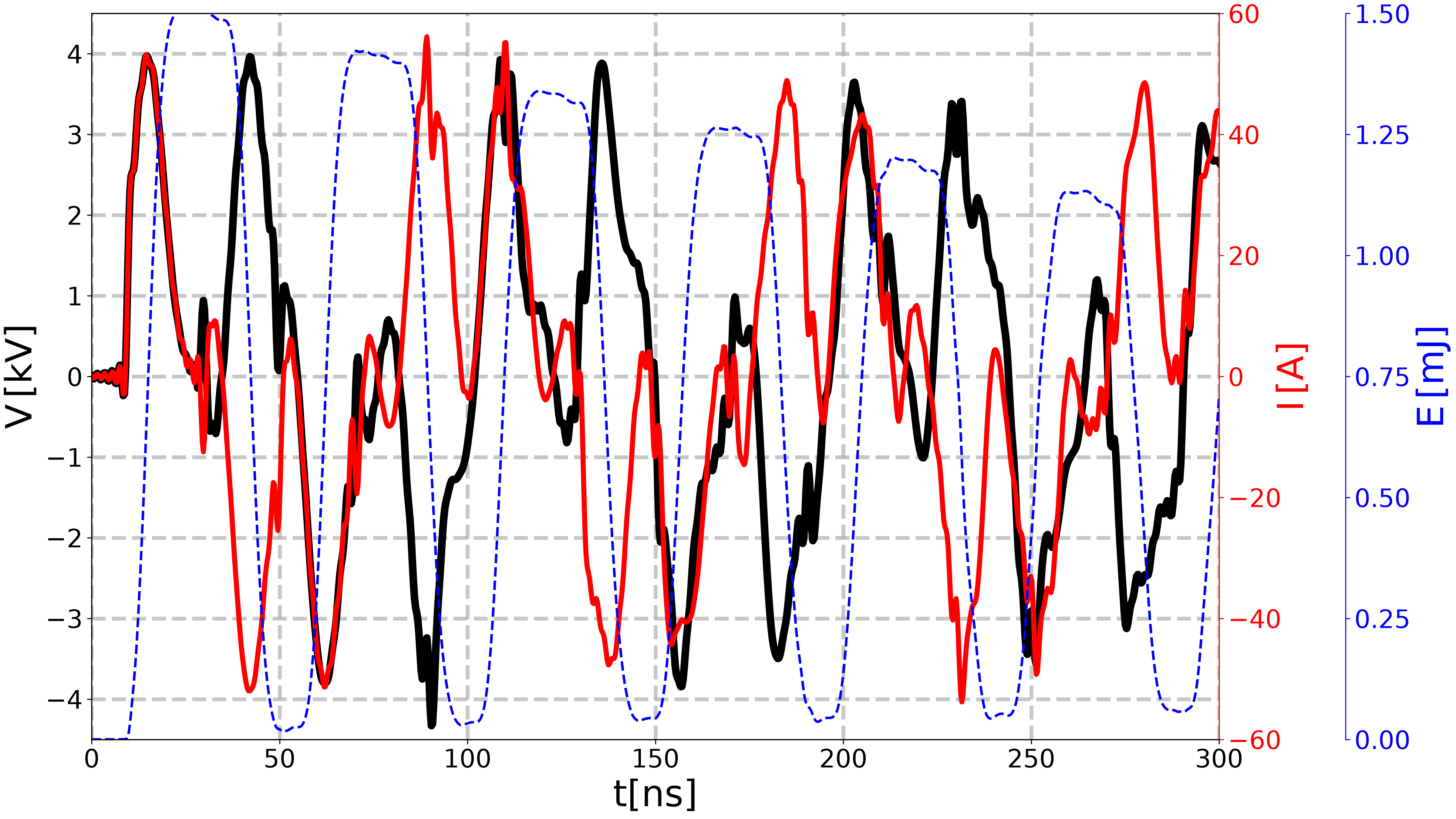
Plotting voltage at x = 2.00 m= 50.00% of the line)
Plotting current at x = 2.00 m= 50.00% of the line)