Determination of cable properties.

This example shows how to determine the properties of a coaxial cable from experimental data, and compare them to the datasheet values.

# This sets the third figure as the thumbnail for the example gallery.
# sphinx_gallery_thumbnail_number = 3
# This displays each image separately in the example gallery.
# sphinx_gallery_multi_image = "single"

First, we import the required libraries.

We start by importing the modules we need:

• matplotlib for drawing graphs,

• numpy for array functions,

• pyresiflex for the generator, load and transmission line.

import matplotlib.pyplot as plt
import numpy as np
import yaml

import pyresiflex.misc.units as u
from pyresiflex.misc.plot import plot_voltage_current, set_mpl_style
from pyresiflex.misc.utils import get_path_to_data

set_mpl_style(nb_columns=2)

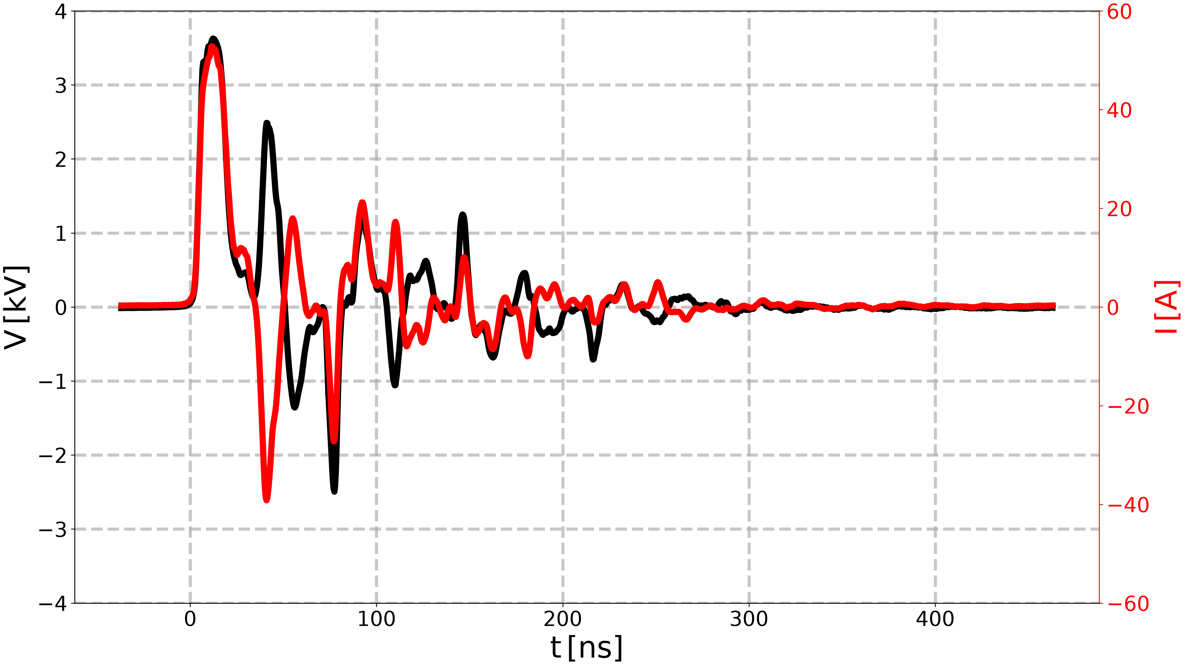
Load [Minesi2022] experimental data of remote configuration.

# Load the raw data from Figure 16 of [Minesi2022]_.
file = get_path_to_data(
    "Minesi2022",
    "fig16_remoteConfiguration.csv",
)
data = np.loadtxt(file, skiprows=3, delimiter=";")
times_raw = data[:, 0] * 1e-9  # [s]
voltages_raw = data[:, 1] * 1e3  # [V]
currents_raw = data[:, 3]  # [A]


# Plot the raw data.
fig, ax_v, ax_i = plot_voltage_current(
    voltage_time=times_raw,
    voltage_value=voltages_raw,
    current_time=times_raw,
    current_value=currents_raw,
)
ax_v.set_ylim(-4, 4)
ax_i.set_ylim(-60, 60)

plt.show()

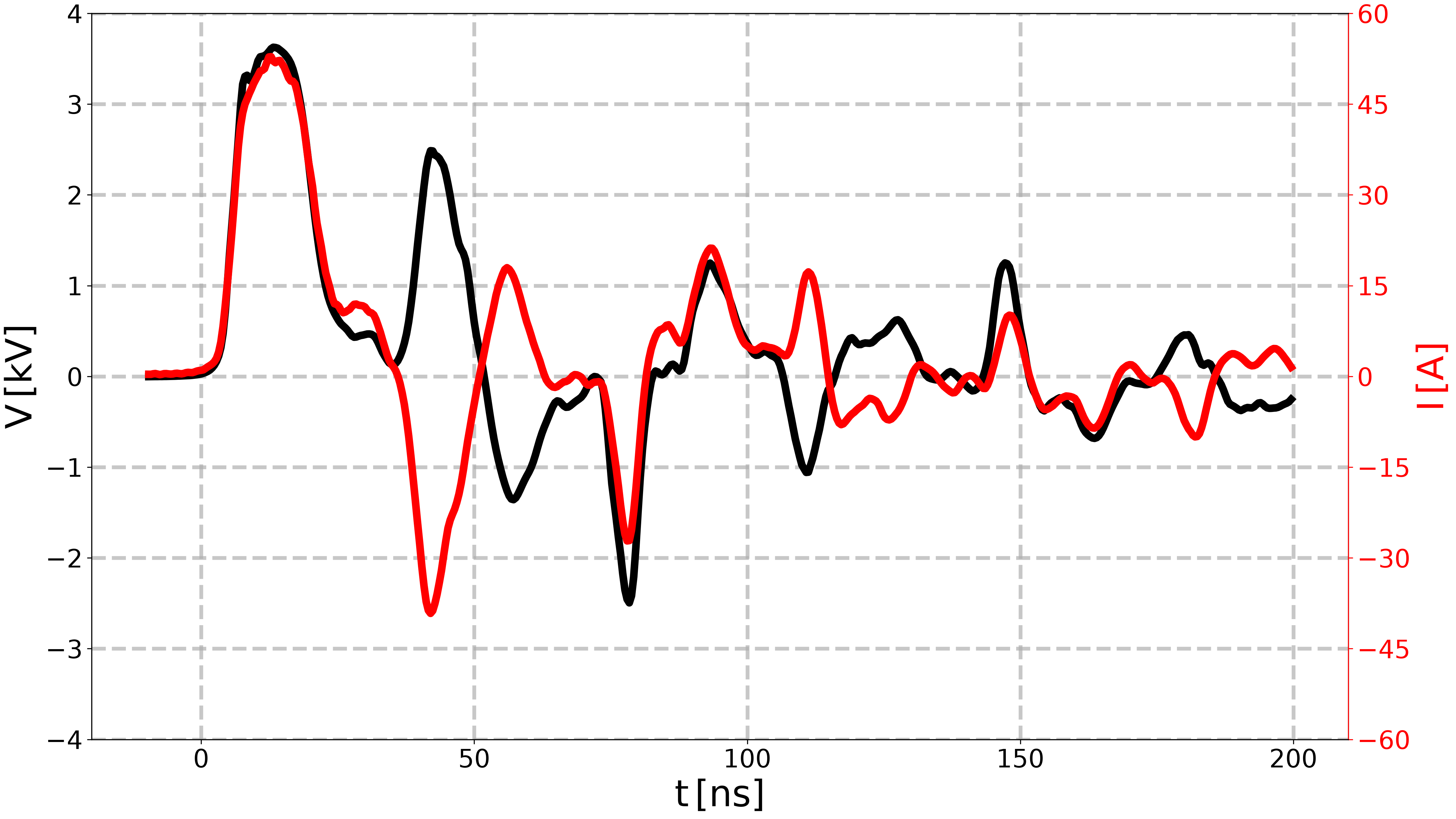
Preprocess the data.

# Define the zero at the first time the voltage reaches `threshold_voltage`.
threshold_voltage = 25  # [V]
idx_first = np.where(np.abs(voltages_raw) > threshold_voltage)[0][0]
times_raw = times_raw - times_raw[idx_first]

# Define a time window to analyze.
lower_time_window = -10e-9  # [s]
upper_time_window = 200e-9  # [s]

# Limit the time window to [lower_time_window, upper_time_window]
idx_min_wanted_time = np.where(times_raw > lower_time_window)[0][0]
idx_max_wanted_time = np.where(times_raw > upper_time_window)[0][0]

# Limit the time, voltages and currents to the wanted period.
times_expe = times_raw[idx_min_wanted_time:idx_max_wanted_time]
voltages_expe = voltages_raw[idx_min_wanted_time:idx_max_wanted_time]
currents_expe = currents_raw[idx_min_wanted_time:idx_max_wanted_time]


# Plot the preprocessed data.
fig, ax_v, ax_i = plot_voltage_current(
    voltage_time=times_expe,
    voltage_value=voltages_expe,
    current_time=times_expe,
    current_value=currents_expe,
)
ax_v.set_ylim(-4, 4)
ax_i.set_ylim(-60, 60)
ax_i.set_yticks([-60, -45, -30, -15, 0, 15, 30, 45, 60])

plt.show()

Determine the time delay between the incident and reflected wave.

# Find the points where the voltage reaches 2 kV.
# Change this value to observe the time delay at different voltage levels.
t_2kV = times_expe[np.where(np.abs(voltages_expe - 2000) < 100)[0]]
print(f"Times when voltage reaches 2 kV: {t_2kV * 1e9} ns")
# Time difference between detection of 2 kV, for the first rising edge.
delta_t = t_2kV[2] - t_2kV[0]  # [s]
print(
    "Time difference between the incident"
    f" and reflected wave: {delta_t * 1e9} ns"
)

fig, ax_v, ax_i = plot_voltage_current(
    voltage_time=times_expe,
    voltage_value=voltages_expe,
    current_time=times_expe,
    current_value=currents_expe,
)
ax_v.set_ylim(-4, 4)
ax_i.set_ylim(-60, 60)
ax_i.set_yticks([-60, -45, -30, -15, 0, 15, 30, 45, 60])

ax_v.axvline(t_2kV[0] * 1e9, color="blue", linestyle="--", lw=3)
ax_v.axvline(t_2kV[2] * 1e9, color="blue", linestyle="--", lw=3)
ax_v.text(
    t_2kV[0] * 1e9,
    -3,
    "Incident wave (2 kV)",
    color="blue",
    ha="center",
    bbox=dict(facecolor="white", alpha=0.7, edgecolor="none"),
)
ax_v.text(
    t_2kV[2] * 1e9,
    3,
    "Reflected wave (2 kV)",
    color="blue",
    ha="center",
    bbox=dict(facecolor="white", alpha=0.7, edgecolor="none"),
)

plt.show()

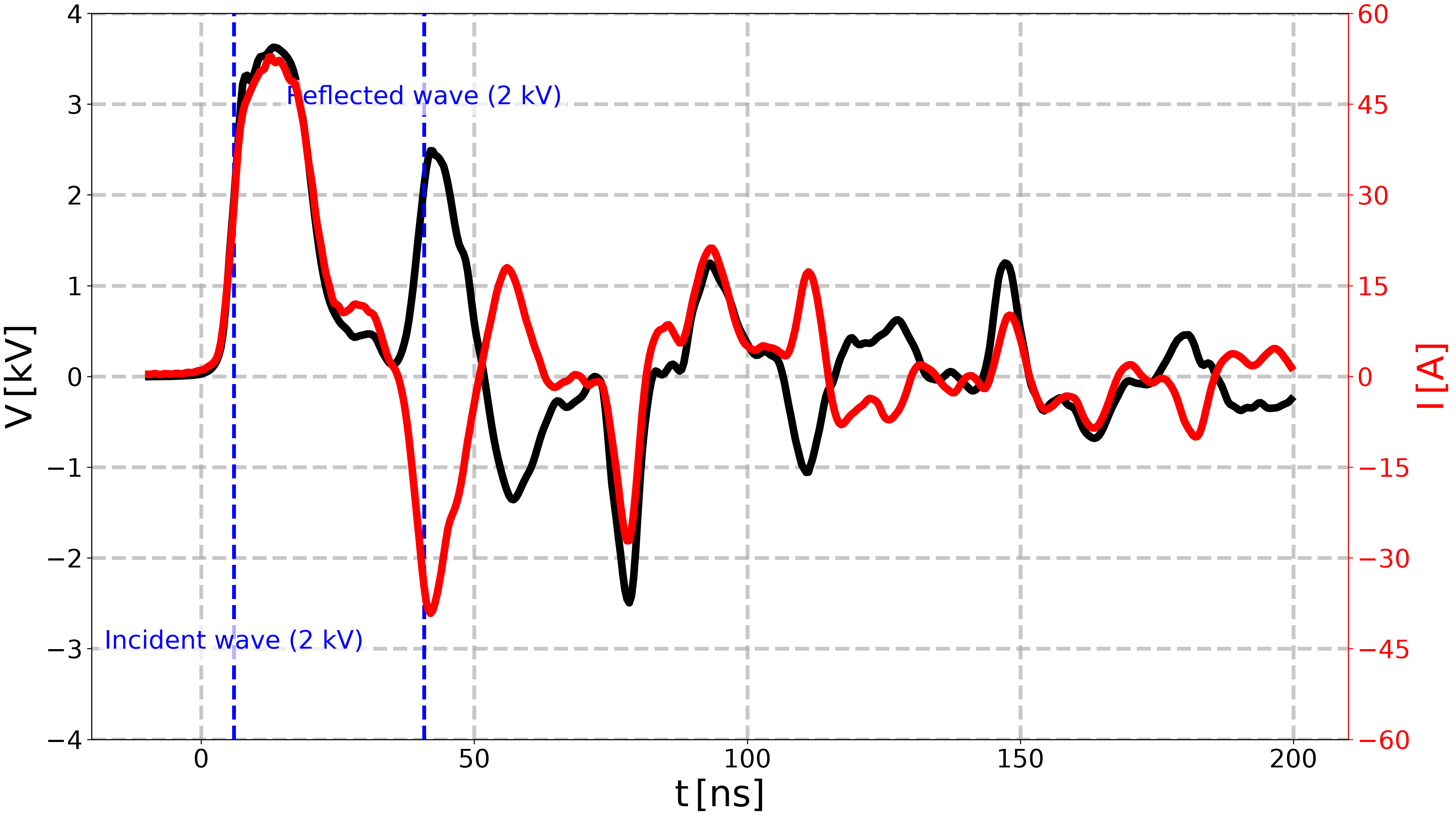
Times when voltage reaches 2 kV: [ 6.  20.4 40.8 45.6] ns
Time difference between the incident and reflected wave: 34.8 ns

Determine the cable properties from the datasheet.

We will use the datasheet to get the celerity and characteristic impedance. We will then use the time delay to get the length of the cable.

# In [Minesi2022]_, the cable used was a AlphaWire 9011A RG11A/U.
# Data come from the datasheet of the AlphaWire 9011A RG11A/U cable,
# in "./src/pyresiflex/data/Minesi2022/Alpha Wire 9011A Tech Data.pdf".
# The cable has the following properties:
c_datasheet = 0.66 * u.c_0  # [m/s]
Z_c_datasheet = 75  # [Ohm]


# We need to make an assumption on the position of the probes.
# Here, we assume that the probes are located at the same position,
# at the middle of the cable.
# x = L / 2
#
# Then, the wave velocity is given by:
#   c = 2 * (L - x) / delta_t
#     = L / delta_t
# Thus, the length of the cable is:
L_from_datasheet = c_datasheet * delta_t  # [m]

Determine the cable properties from the experimental data.

[Minesi2022] provides the cable length used, roughly 6 m. However, there were two cables of 3 m connected in series, via a box, where probes are connected. This box adds some additional length, roughly 0.2 m. Thus, we will assume that the length of the cable is:

L_experimental = 6.2  # [m]
# [Minesi2022]_ also provides the probe positions, at the middle of the cable.
x_experimental = L_experimental / 2  # [m]

# time delay between the incident and reflected wave (for 2 kV).
delta_t = 34.8e-9  # [s]
# Uncertainties on the measurements:
# .. Uncertainty on the length of the cable, due to the box.
ΔL_expe = 0.1  # [m]
# .. Uncertainty on the position of the probes, due to the box.
Δx_expe = 0.1  # [m]
# .. Uncertainty on the time delay, after playing with the threshold voltage.
Δdelta_t = 1e-9  # [s]

# Then, the wave velocity is given by:
c_experimental = 2 * (L_experimental - x_experimental) / delta_t
# .. Uncertainty on the wave velocity, using error propagation:
Δc_experimental = c_experimental * np.sqrt(
    (ΔL_expe / (L_experimental - x_experimental)) ** 2
    + (Δx_expe / (L_experimental - x_experimental)) ** 2
    + (Δdelta_t / delta_t) ** 2
)

print(
    f"Experimental celerity: {c_experimental:.2e} m/s"
    f" ± {Δc_experimental:.2e} m/s"
)

# The characteristic impedance can be determined from the maximum voltage
# and current of the incident wave:
max_voltage = np.max(voltages_expe)
max_current = np.max(currents_expe)
Z_c = max_voltage / max_current
Δmax_voltage = 100  # [V]
Δmax_current = 1  # [A]
ΔZ_c = Z_c * np.sqrt(
    (Δmax_voltage / max_voltage) ** 2 + (Δmax_current / max_current) ** 2
)
print(
    f"Experimental maximum voltage: {max_voltage:.2f} V ± {Δmax_voltage:.2f} V"
)
print(
    f"Experimental maximum current: {max_current:.2f} A ± {Δmax_current:.2f} A"
)
print(f"Experimental characteristic impedance: {Z_c:.2f} Ω ± {ΔZ_c:.2f} Ω")

Experimental celerity: 1.78e+08 m/s ± 9.61e+06 m/s
Experimental maximum voltage: 3626.63 V ± 100.00 V
Experimental maximum current: 52.84 A ± 1.00 A
Experimental characteristic impedance: 68.63 Ω ± 2.30 Ω

Compare the results.

print("Cable properties from datasheet:")
print(f"  Length: {L_from_datasheet:.2f} m")
print(f"  Celerity: {c_datasheet / u.c_0:.2f} c = {c_datasheet:.2e} m/s")
print(f"  Characteristic impedance: {Z_c_datasheet:.2f} Ω")
print("")
print("Cable properties from experimental data:")
print(f"  Length: {L_experimental:.2f} m ± {ΔL_expe:.2f} m")
print(
    f"  Celerity: {c_experimental / u.c_0:.2f} c ="
    f" {c_experimental:.2e} m/s ± {Δc_experimental:.2e} m/s"
)
print(f"  Characteristic impedance: {Z_c:.2f} Ω ± {ΔZ_c:.2f} Ω")

Cable properties from datasheet:
  Length: 6.89 m
  Celerity: 0.66 c = 1.98e+08 m/s
  Characteristic impedance: 75.00 Ω

Cable properties from experimental data:
  Length: 6.20 m ± 0.10 m
  Celerity: 0.59 c = 1.78e+08 m/s ± 9.61e+06 m/s
  Characteristic impedance: 68.63 Ω ± 2.30 Ω

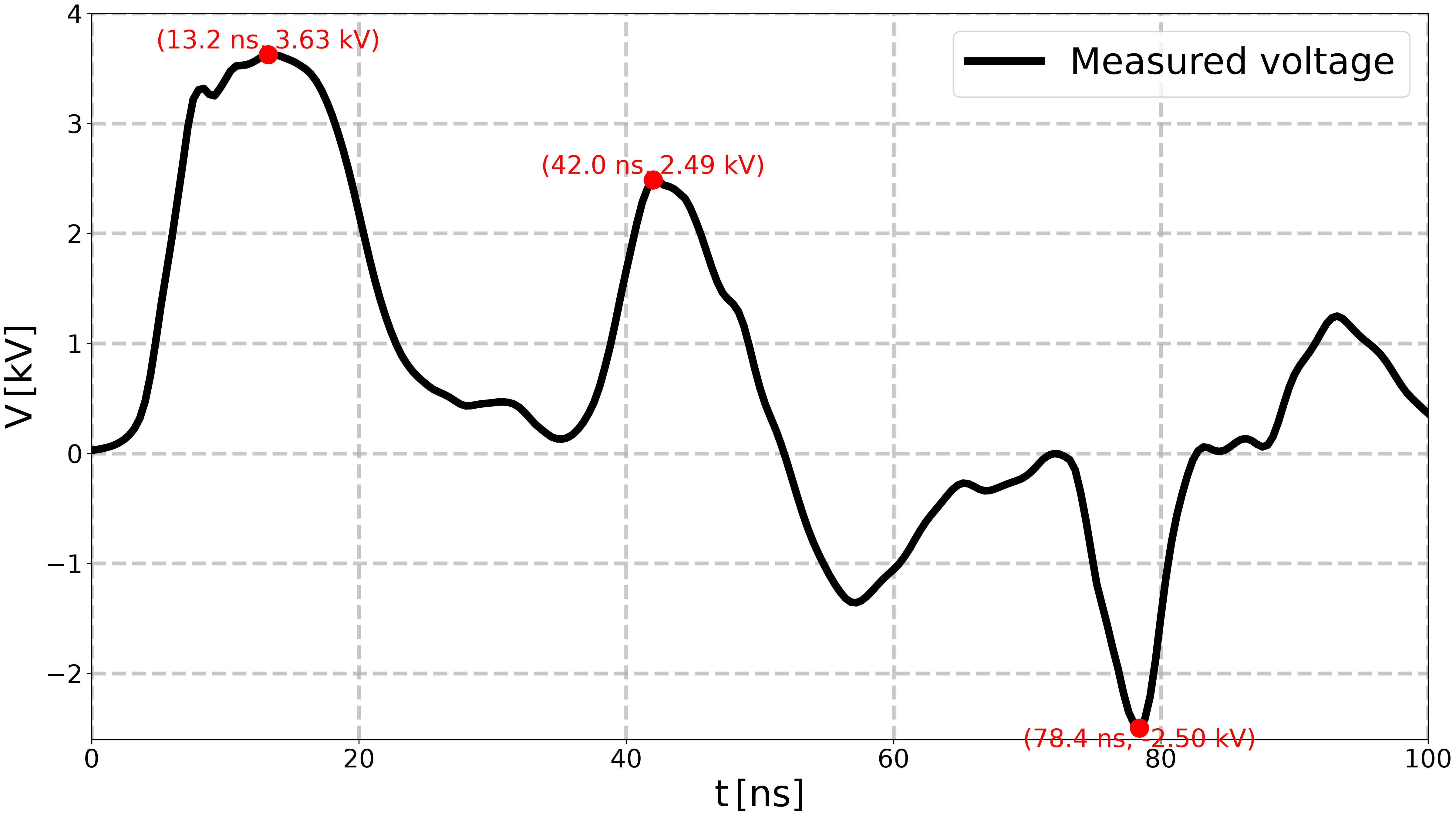
Determine the internal resistance of the generator.

# Time windows for the first incident pulse, the first reflected pulse,
# and the second incident pulse.
pulse_1i_mask = (times_expe >= 0) & (times_expe <= 35e-9)
pulse_1r_mask = (times_expe >= 35e-9) & (times_expe <= 70e-9)
pulse_2i_mask = (times_expe >= 70e-9) & (times_expe <= 105e-9)

# Compute max voltage on these time windows, and associated times.
max_voltage_1i = np.max(np.abs(voltages_expe[pulse_1i_mask]))
max_voltage_1r = np.max(np.abs(voltages_expe[pulse_1r_mask]))
max_voltage_2i = np.max(np.abs(voltages_expe[pulse_2i_mask]))
idx_max_voltage_1i = np.argmax(np.abs(voltages_expe[pulse_1i_mask]))
idx_max_voltage_1r = np.argmax(np.abs(voltages_expe[pulse_1r_mask]))
idx_max_voltage_2i = np.argmax(np.abs(voltages_expe[pulse_2i_mask]))
time_max_voltage_1i = times_expe[pulse_1i_mask][idx_max_voltage_1i]
time_max_voltage_1r = times_expe[pulse_1r_mask][idx_max_voltage_1r]
time_max_voltage_2i = times_expe[pulse_2i_mask][idx_max_voltage_2i]
sign_1i = np.sign(voltages_expe[pulse_1i_mask][idx_max_voltage_1i])
sign_1r = np.sign(voltages_expe[pulse_1r_mask][idx_max_voltage_1r])
sign_2i = np.sign(voltages_expe[pulse_2i_mask][idx_max_voltage_2i])

# Plot the voltage signal and the max voltages on the three pulses.
fig, ax = plt.subplots()
ax.plot(
    times_expe * 1e9,
    voltages_expe * 1e-3,
    color="black",
    label="Measured voltage",
)
for time, voltage, sign in zip(
    [time_max_voltage_1i, time_max_voltage_1r, time_max_voltage_2i],
    [max_voltage_1i, max_voltage_1r, max_voltage_2i],
    [sign_1i, sign_1r, sign_2i],
):
    ax.scatter(
        time * 1e9,
        voltage * sign * 1e-3,
        color="red",
        s=200,
        zorder=3,
    )
    ax.text(
        time * 1e9,
        voltage * sign * 1e-3,
        f"({time * 1e9:.1f} ns, {voltage * sign * 1e-3:.2f} kV)",
        color="red",
        ha="center",
        va="bottom" if sign > 0 else "top",
    )


ax.set_xlabel(r"$\mathregular{t \, [ns]}$")
ax.set_ylabel(r"$\mathregular{V \, [kV]}$")
ax.set_xlim(0, 100)
ax.set_ylim(-2.6, 4)
ax.legend()

plt.show()


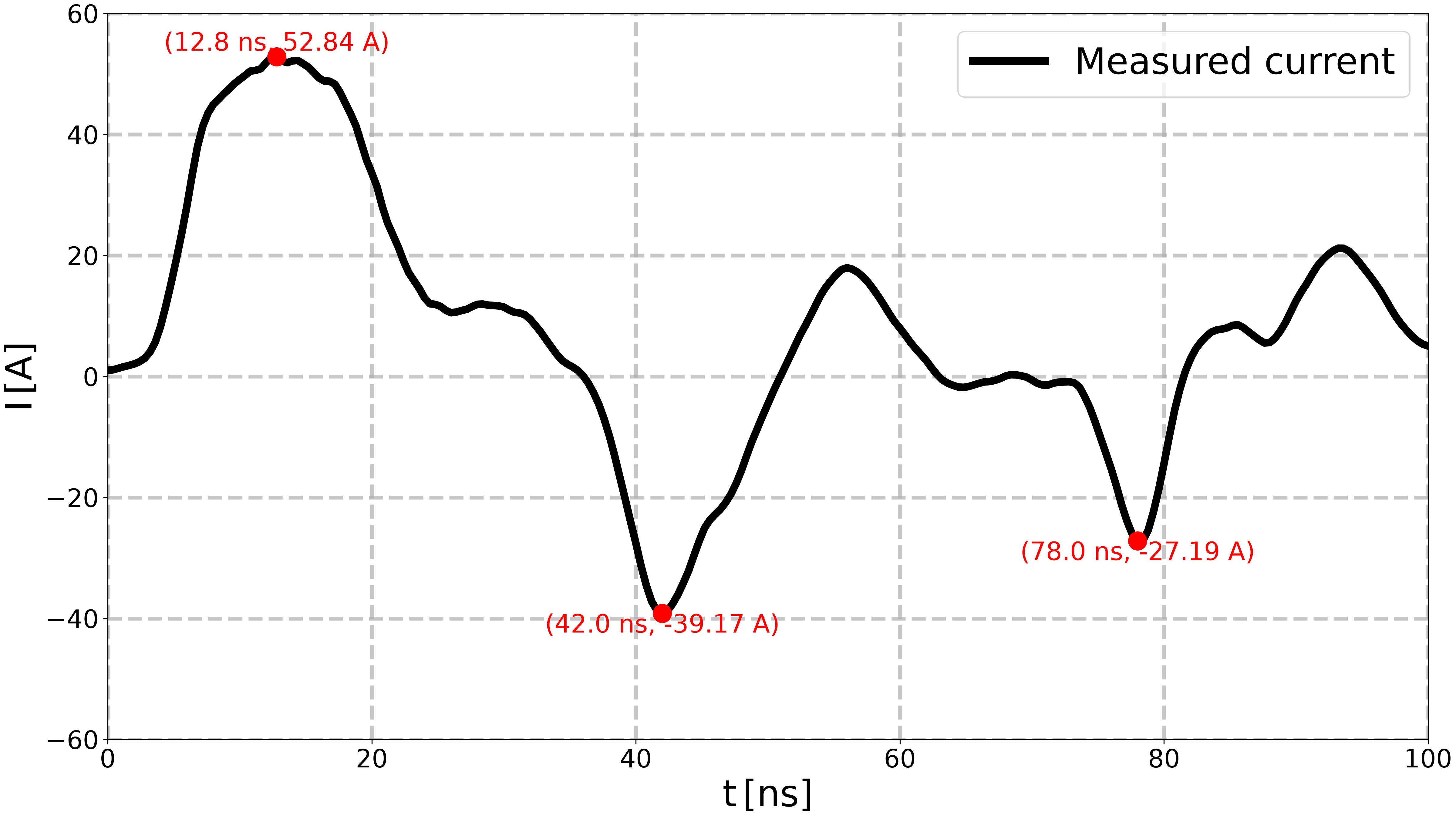
# Do the same, but with current instead of voltage.
# Compute max current on the time windows, and associated times.
max_current_1i = np.max(np.abs(currents_expe[pulse_1i_mask]))
max_current_1r = np.max(np.abs(currents_expe[pulse_1r_mask]))
max_current_2i = np.max(np.abs(currents_expe[pulse_2i_mask]))
idx_max_current_1i = np.argmax(np.abs(currents_expe[pulse_1i_mask]))
idx_max_current_1r = np.argmax(np.abs(currents_expe[pulse_1r_mask]))
idx_max_current_2i = np.argmax(np.abs(currents_expe[pulse_2i_mask]))
time_max_current_1i = times_expe[pulse_1i_mask][idx_max_current_1i]
time_max_current_1r = times_expe[pulse_1r_mask][idx_max_current_1r]
time_max_current_2i = times_expe[pulse_2i_mask][idx_max_current_2i]
sign_1i = np.sign(currents_expe[pulse_1i_mask][idx_max_current_1i])
sign_1r = np.sign(currents_expe[pulse_1r_mask][idx_max_current_1r])
sign_2i = np.sign(currents_expe[pulse_2i_mask][idx_max_current_2i])

fig, ax = plt.subplots()
ax.plot(
    times_expe * 1e9,
    currents_expe,
    color="black",
    label="Measured current",
)
for time, current, sign in zip(
    [time_max_current_1i, time_max_current_1r, time_max_current_2i],
    [max_current_1i, max_current_1r, max_current_2i],
    [sign_1i, sign_1r, sign_2i],
):
    ax.scatter(
        time * 1e9,
        current * sign,
        color="red",
        s=200,
        zorder=3,
    )
    ax.text(
        time * 1e9,
        current * sign,
        f"({time * 1e9:.1f} ns, {current * sign:.2f} A)",
        color="red",
        ha="center",
        va="bottom" if sign > 0 else "top",
    )

ax.set_xlabel(r"$\mathregular{t \, [ns]}$")
ax.set_ylabel(r"$\mathregular{I \, [A]}$")
ax.set_xlim(0, 100)
ax.set_ylim(-60, 60)
ax.legend()
plt.show()


# Now, we can compute the resistance, either from voltage or from current:
Rg_voltage = (
    Z_c * (max_voltage_1r - max_voltage_2i) / (max_voltage_1r + max_voltage_2i)
)
Rg_current = (
    Z_c * (max_current_1r - max_current_2i) / (max_current_1r + max_current_2i)
)
print(f"Internal resistance of the generator from voltage: {Rg_voltage:.2f} Ω")
print(f"Internal resistance of the generator from current: {Rg_current:.2f} Ω")
# Note that the value of Rg_voltage is negative, which is not physical.
# This is due to the fact that the max voltage of the reflected pulse is
# slightly higher than the max voltage of the second incident pulse,
# which can be explained by measurement uncertainties.
# We will therefore use the value of Rg_current for the rest of the example.

# Evaluation of the incertitude on Rg:
I_1r = max_current_1r
I_2i = max_current_2i
ΔI_1r = 1  # [A]
ΔI_2i = 1  # [A]
print(f"Experimental maximum current: {max_current_1r:.2f} A ± {ΔI_1r:.2f} A")
print(f"Experimental maximum current: {max_current_2i:.2f} A ± {ΔI_2i:.2f} A")

ΔR_g = Rg_current * np.sqrt(
    (ΔZ_c / Z_c) ** 2
    + 4
    * ((I_2i * ΔI_1r) ** 2 + (I_1r * ΔI_2i) ** 2)
    / ((I_1r) ** 2 - (I_2i) ** 2) ** 2
)
print(
    "Estimated internal resistance of the generator:"
    f" {Rg_current:.2f} ± {ΔR_g:.2f} Ω"
)


# Computation of the attenuation factor between the generator and the cable:
alpha_g = Z_c / (Z_c + Rg_current)
print(f"Attenuation factor between the generator and the cable: {alpha_g:.2f}")

Δalpha_g = (
    alpha_g**3 / Z_c * np.sqrt((ΔR_g) ** 2 + (ΔZ_c * Rg_current / Z_c) ** 2)
)
print(
    "Estimated attenuation factor between the generator and the cable:"
    f" {alpha_g:.2f} ± {Δalpha_g:.2f}"
)

• 
• 

Internal resistance of the generator from voltage: -0.12 Ω
Internal resistance of the generator from current: 12.39 Ω
Experimental maximum current: 39.17 A ± 1.00 A
Experimental maximum current: 27.19 A ± 1.00 A
Estimated internal resistance of the generator: 12.39 ± 1.54 Ω
Attenuation factor between the generator and the cable: 0.85
Estimated attenuation factor between the generator and the cable: 0.85 ± 0.01

Write experimental results to a .yaml file.

experimental_results = {
    "description": (
        "Cable properties determined from Minesi2022 experiments,"
        " with the assumption that the probes are located at the middle"
        " of the transmission line."
    ),
    "celerity": {
        "value": float(c_experimental),
        "uncertainty": float(Δc_experimental),
    },
    "characteristic_impedance": {
        "value": float(Z_c),
        "uncertainty": float(ΔZ_c),
    },
    "length": {"value": float(L_experimental), "uncertainty": float(ΔL_expe)},
    "x_meas": {"value": float(x_experimental), "uncertainty": float(Δx_expe)},
    "internal_resistance_generator": {
        "value": float(Rg_current),
        "uncertainty": float(ΔR_g),
    },
    "attenuation_factor_generator_cable": {
        "value": float(alpha_g),
        "uncertainty": float(Δalpha_g),
    },
}
with open(
    get_path_to_data("Minesi2022", "cable_properties.yaml", force_return=True),
    "w",
    encoding="utf-8",
) as file:
    yaml.dump(
        experimental_results,
        file,
        encoding="utf-8",
        sort_keys=False,
        # Do not wrap long lines (e.g. the description), so the output
        # matches the format enforced by the `pretty-format-yaml` hook.
        width=float("inf"),
    )

Determining if the cable can be considered perfect or not.

Data come from the datasheet of the AlphaWire 9011A RG11A/U cable, in “./src/pyresiflex/data/Minesi2022/Alpha Wire 9011A Tech Data.pdf”.

# feet to meters conversion: 1 ft = 0.3048 m
feet_to_m = 0.3048  # [m/ft]

print("Cable properties from datasheet:")
# Inner conductor resistance per unit length:
R_ohm_feet = 6.3 / 1000  # [Ω/ft]
R_ohm_m = R_ohm_feet / feet_to_m  # [Ω/m]
print(f"Cable resistance: {R_ohm_m * 1e3:.1f} Ω/km")

# Velocity of propagation:
c = 0.66 * u.c_0  # [m/s] (from datasheet)

# Ground capacitance per unit length:
C_F_per_feet = 20.5e-12  # [F/ft]
C_F_per_m = C_F_per_feet / feet_to_m  # [F/m]
print(f"Cable capacitance: {C_F_per_m * 1e12:.1f} pF/m")

# Inductance per unit length:
# (Assuming a lossless cable, to derive the inductance from the capacitance
# and the velocity of propagation)
L_H_per_m = 1 / (c**2 * C_F_per_m)  # [H/m]
print(f"Cable inductance: {L_H_per_m * 1e9:.1f} nH/m")


# Cable attenuation:
alpha_dB_per_ft = [
    5.2 / 100,  # [dB/ft] at 400 MHz
    9.4 / 100,  # [dB/ft] at 1 GHz
]
alpha_dB_per_m = [a / feet_to_m for a in alpha_dB_per_ft]  # [dB/m]
f_attenuation = [400e6, 1e9]  # [Hz]
print(f"Cable attenuation: {alpha_dB_per_m[0]:.2f} dB/m at 400 MHz")
print(f"Cable attenuation: {alpha_dB_per_m[1]:.2f} dB/m at 1 GHz")
# Create a function to (linearly) interpolate the attenuation at any frequency.
alpha_dB_per_m_func = np.polynomial.polynomial.polyfit(
    x=f_attenuation, y=alpha_dB_per_m, deg=1
)

for f in [0, 100e6, 200e6, 300e6, 400e6, 600e6, 800e6, 1e9]:
    print(
        f"  at {f / 1e6:.0f} MHz: "
        f"{np.polynomial.polynomial.polyval(f, alpha_dB_per_m_func):.2f} dB/m"
    )


# Trapezoidal pulse parameters:
print("-" * 40)
print("Trapezoidal pulse parameters:")
t_rising = 2e-9  # [s]
f_rising = 0.35 / t_rising  # [Hz]
t_flat = 10e-9  # [s]
f_flat = 1 / t_flat  # [Hz]
print(f"Rising edge frequency: {f_rising / 1e6:.1f} MHz")
print(f"Flat top frequency: {f_flat / 1e6:.1f} MHz")

# Attenuation at the rising edge frequency:
alpha_rising = np.polynomial.polynomial.polyval(
    f_rising, alpha_dB_per_m_func
)  # [dB/m]
# Attenuation at the flat top frequency:
alpha_flat = np.polynomial.polynomial.polyval(
    f_flat, alpha_dB_per_m_func
)  # [dB/m]
print(f"Cable attenuation at rising edge frequency: {alpha_rising:.2f} dB/m")
print(f"Cable attenuation at flat top frequency: {alpha_flat:.2f} dB/m")

# Attenuation over the whole cable length:
print("-" * 40)
for L in [10, 24]:  # [m]
    print(f"Attenuation of voltage over {L} m of cable:")
    total_attenuation = 10 ** (-alpha_rising * L / 20)
    print(f"  at rising edge frequency: {total_attenuation:.3f} (-)")
    total_attenuation = 10 ** (-alpha_flat * L / 20)
    print(f"  at flat top frequency: {total_attenuation:.3f} (-)")

Cable properties from datasheet:
Cable resistance: 20.7 Ω/km
Cable capacitance: 67.3 pF/m
Cable inductance: 379.8 nH/m
Cable attenuation: 0.17 dB/m at 400 MHz
Cable attenuation: 0.31 dB/m at 1 GHz
  at 0 MHz: 0.08 dB/m
  at 100 MHz: 0.10 dB/m
  at 200 MHz: 0.12 dB/m
  at 300 MHz: 0.15 dB/m
  at 400 MHz: 0.17 dB/m
  at 600 MHz: 0.22 dB/m
  at 800 MHz: 0.26 dB/m
  at 1000 MHz: 0.31 dB/m
----------------------------------------
Trapezoidal pulse parameters:
Rising edge frequency: 175.0 MHz
Flat top frequency: 100.0 MHz
Cable attenuation at rising edge frequency: 0.12 dB/m
Cable attenuation at flat top frequency: 0.10 dB/m
----------------------------------------
Attenuation of voltage over 10 m of cable:
  at rising edge frequency: 0.872 (-)
  at flat top frequency: 0.890 (-)
Attenuation of voltage over 24 m of cable:
  at rising edge frequency: 0.720 (-)
  at flat top frequency: 0.755 (-)