Comparison of electron density results between electrical and optical methods.#
This example shows how to compute electron density in a plasma from electrical measurements, and compare it with experimental data obtained via Optical Emission Spectroscopy (OES).
In this example, the plasma is assumed to be a time-varying resistance.
Experimental data of [Minesi2022] are used to extract the plasma resistance, as well as the electric field in the plasma.
This electric field is then used to get the electron mobility vs time. This mobility was computed with Bolsig+ beforehand, versus reduced electric field.
The electron density is then computed from the plasma resistance and the mobility, and compared to experimental data from OES measurements provided by [Minesi2022].
# This sets the third figure as the thumbnail for the example gallery.
# sphinx_gallery_thumbnail_number = 13
# This displays each image separately in the example gallery.
# sphinx_gallery_multi_image = "single"
First, we import the required libraries.#
We start by importing the modules we need:
matplotlib for drawing graphs,
numpy for array functions,
pyresiflex for the generator, load and transmission line.
from dataclasses import dataclass
from pathlib import Path

import matplotlib.pyplot as plt
import numpy as np

from pyresiflex.cable.cable import PerfectCable
from pyresiflex.experiment.purely_resistive_experiment import (
    PurelyResistiveExperiment,
)
from pyresiflex.generator.generator_real_impedance import (
    FromMeasurementGenerator,
)
from pyresiflex.misc.load_data import load_minesi_data
from pyresiflex.misc.plot import plot_voltage_current, set_mpl_style
from pyresiflex.misc.units import e, k_b
from pyresiflex.misc.utils import get_path_to_data
from pyresiflex.solver.purely_resistive_solution import PurelyResistiveSolution

set_mpl_style(nb_columns=2)
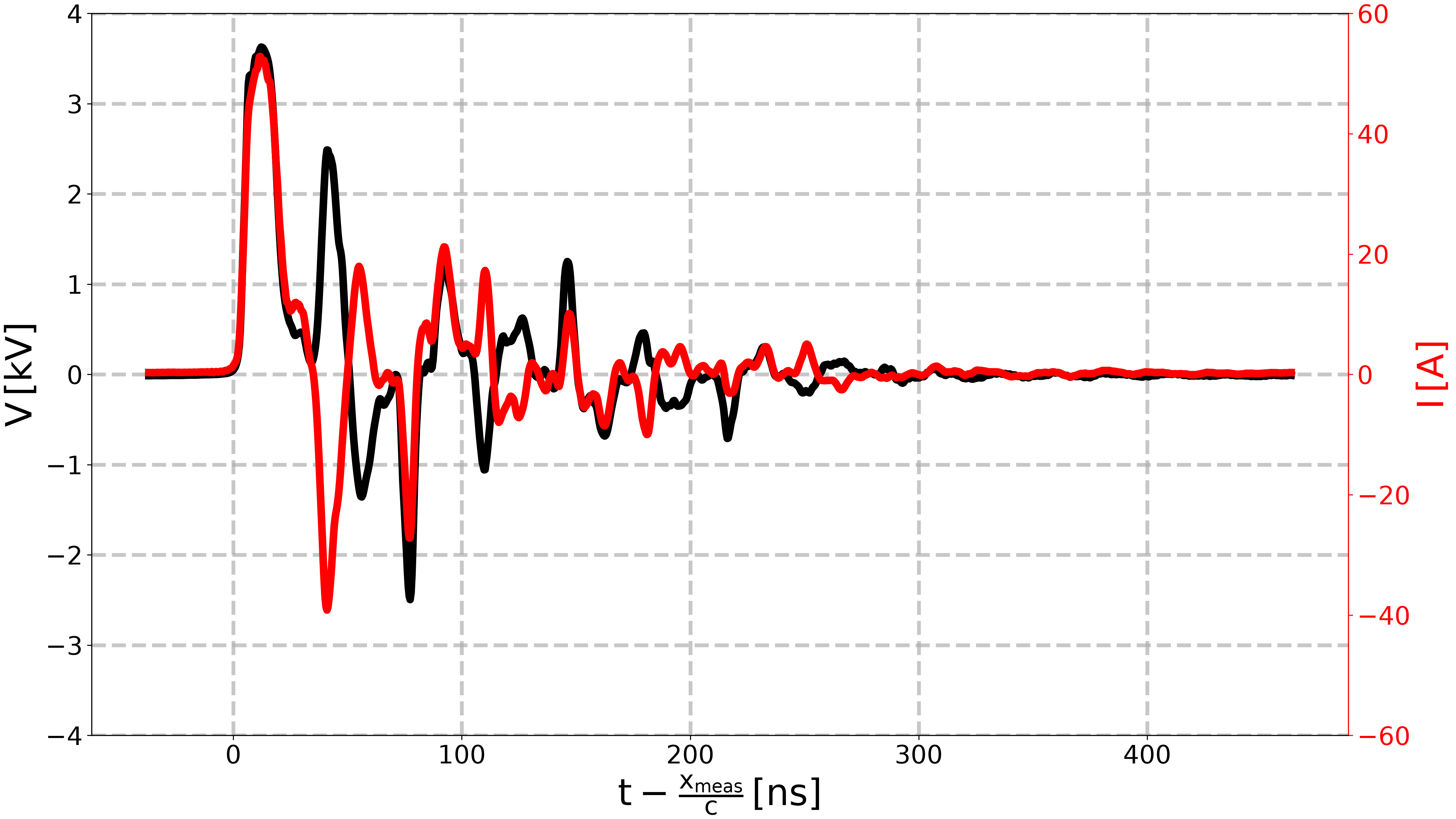
Load [Minesi2022] experimental data of remote configuration.#
# Load the raw data from Figure 16 of [Minesi2022]_.
file = get_path_to_data(
    "Minesi2022",
    "fig16_remoteConfiguration.csv",
)
raw_data = np.loadtxt(file, skiprows=3, delimiter=";")
times_raw = raw_data[:, 0] * 1e-9  # [s]
voltages_raw = raw_data[:, 1] * 1e3  # [V]
currents_raw = raw_data[:, 3]  # [A]

# Plot the raw data.
fig, ax_v, ax_i = plot_voltage_current(
    voltage_time=times_raw,
    voltage_value=voltages_raw,
    current_time=times_raw,
    current_value=currents_raw,
)
ax_v.set_xlabel(r"$\mathregular{t - \frac{x_{meas}}{c} \, [ns]}$")
ax_v.set_ylim(-4, 4)
ax_i.set_ylim(-60, 60)

plt.show()
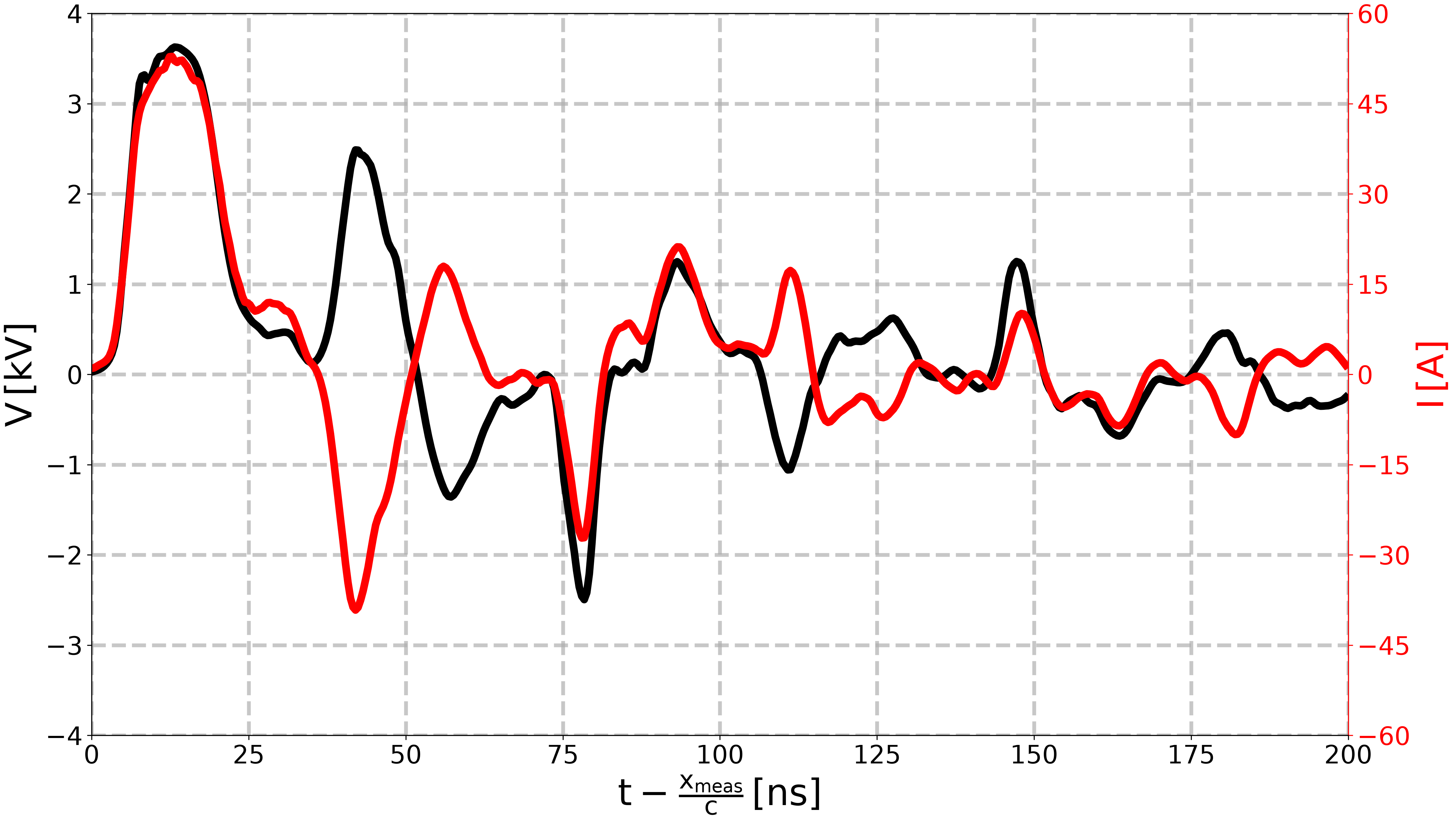
Preprocess the data.#
# Define the zero at the first time the voltage reaches `threshold_voltage`.
threshold_voltage = 25  # [V]
idx_first = np.where(np.abs(voltages_raw) > threshold_voltage)[0][0]
times_raw = times_raw - times_raw[idx_first]

# Define a time window to analyze.
lower_time_window = -20e-9  # [s]
upper_time_window = 200e-9  # [s]

# Limit the time window to [lower_time_window, upper_time_window]
idx_min_wanted_time = np.where(times_raw > lower_time_window)[0][0]
idx_max_wanted_time = np.where(times_raw > upper_time_window)[0][0]

# Limit the time, voltages and currents to the wanted period.
times_expe = times_raw[idx_min_wanted_time:idx_max_wanted_time]
voltages_expe = voltages_raw[idx_min_wanted_time:idx_max_wanted_time]
currents_expe = currents_raw[idx_min_wanted_time:idx_max_wanted_time]

# Compute the energy from the voltage and current.
energies_expe = np.zeros_like(times_expe)  # [J]
for i in range(len(times_expe)):
    energies_expe[i] = np.trapezoid(
        voltages_expe[:i] * currents_expe[:i], times_expe[:i]
    )


# Plot the preprocessed data.
fig, ax_v, ax_i = plot_voltage_current(
    voltage_time=times_expe,
    voltage_value=voltages_expe,
    current_time=times_expe,
    current_value=currents_expe,
)
ax_v.set_xlabel(r"$\mathregular{t - \frac{x_{meas}}{c} \, [ns]}$")
ax_v.set_xlim(0, 200)
ax_v.set_ylim(-4, 4)
ax_i.set_ylim(-60, 60)
ax_i.set_yticks([-60, -45, -30, -15, 0, 15, 30, 45, 60])

plt.show()
Transmission line parameters.#
# Transmission line parameters estimated from experimental data.
# See `plot_determine_Minesi2022_parameters.py` example for more details.
data = load_minesi_data()

# Length of the transmission line
L = data.L  # [m]
# Measurement points = probe positions
x = data.x_meas  # [m]
# Here, we assume that the probes are located at the same position.
x_meas_voltage = x_meas_current = x  # [m]
# Velocity of propagation of the wave in the cable.
c = data.c  # [m/s]
# Cable characteristic impedance.
Z_c = data.Z_c  # [Ohm]

cable = PerfectCable(
    L=L,
    Z_c=Z_c,
    c=c,
)
Generator parameters.#
# Impedance of the generator.
R_g = data.R_g  # [Ohm]
# Attenuation coefficient.
alpha_g = data.alpha_g  # [-]
# Pulse duration.
pulse_duration = 35e-9  # [s]


def V_meas_generator(t, times, voltages):
    if t < 0:
        return 0.0
    elif t > pulse_duration:
        return 0.0
    else:
        return np.interp(t, times, voltages) / alpha_g


generator = FromMeasurementGenerator(
    R_g=R_g, V_meas=lambda t: V_meas_generator(t, times_expe, voltages_expe)
)

# Plot the voltage signal.
set_mpl_style(nb_columns=1)
fig, ax = plt.subplots()
ax.plot(
    times_expe * 1e9,
    voltages_expe * 1e-3,
    color="black",
    label="Measured voltage",
)
ax.plot(
    times_expe * 1e9,
    [generator.generator_voltage(t) * 1e-3 for t in times_expe],
    "--",
    label="Model generator",
    color="red",
)
ax.set_xlabel(r"$\mathregular{t \, [ns]}$")
ax.set_ylabel(r"$\mathregular{V_g \, [kV]}$")
ax.set_xlim(0, 50)
ax.set_ylim(-0.1, 4.5)
ax.legend()
plt.show()
Plasma parameters.#
expe = PurelyResistiveExperiment(
    experimental_voltage_time=times_expe,
    experimental_voltage_value=voltages_expe,
    x_meas_voltage=x_meas_voltage,
    experimental_current_time=times_expe,
    experimental_current_value=currents_expe,
    x_meas_current=x_meas_current,
    L=L,
    Z_c=Z_c,
    c=c,
    correct_time_zero=True,
)

threshold_voltage_for_resistance = 0.2 * np.max(voltages_expe)  # [V]
expe.compute_plasma_resistance_from_vmeas_and_imeas(
    times_expe,
    threshold=threshold_voltage_for_resistance,
    channel_formation_time=42e-9,
)

plasma_load = expe.load_corrected

# Plot the plasma resistance.
set_mpl_style(nb_columns=1)
fig, ax = expe.plot_resistance(times=times_expe)
ax.set_xlim(0, 200)
ax.set_ylim(-100, 1000)
plt.show()

Solution object.#
solution = PurelyResistiveSolution(
    generator=generator,
    load=plasma_load,
    cable=cable,
)
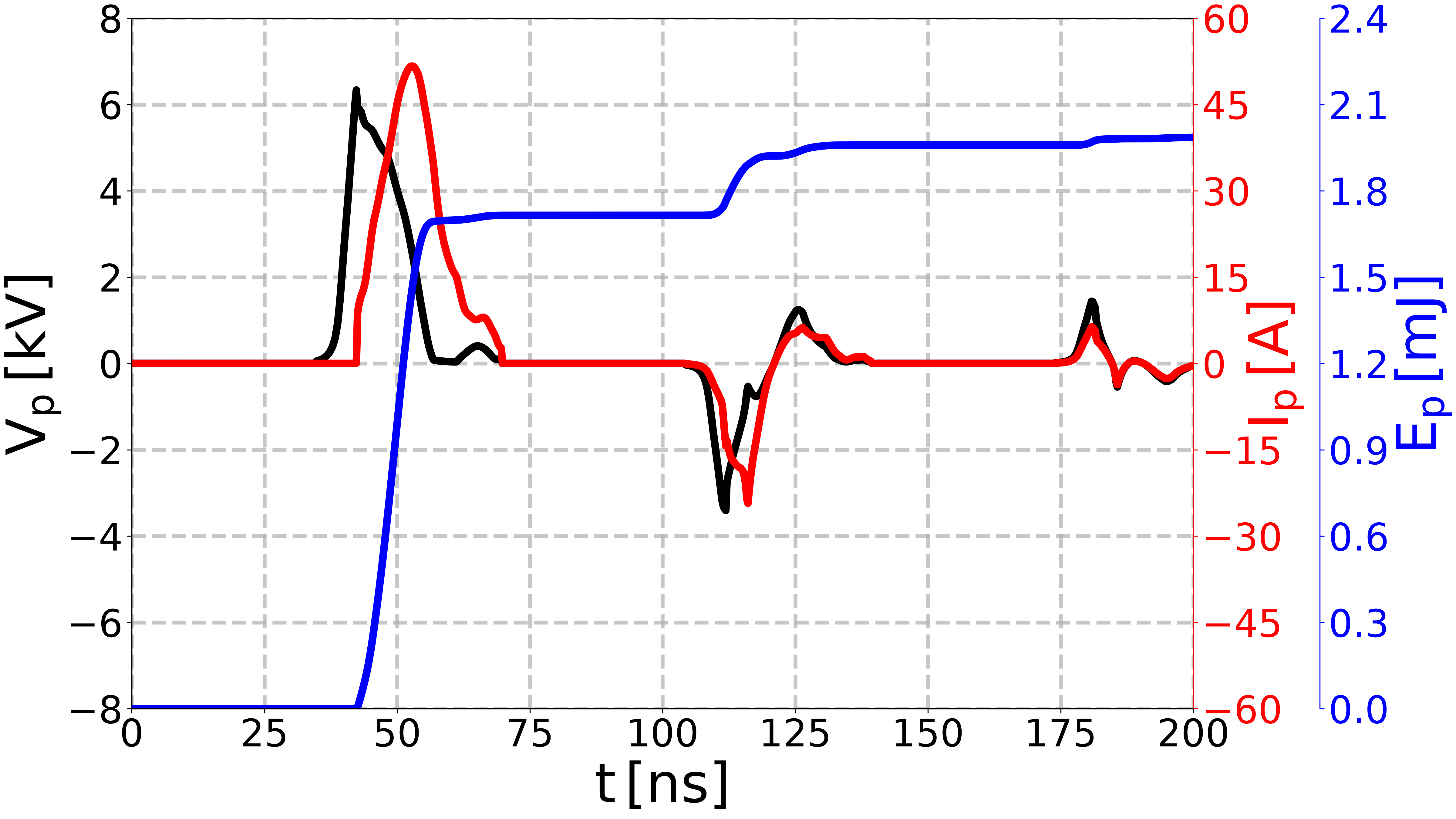
Compute voltage, current and energy at plasma position.#
# Time vector for the simulation.
nb_steps = 1000
times = np.linspace(lower_time_window, upper_time_window, nb_steps)  # [s]
# Position of probes for plasma position.
x = L  # [m]

# Compute the voltage and current at plasma position.
solution.solve(x, times)

plasma_voltage = solution.voltage  # [V]
plasma_current = solution.current  # [A]
plasma_energy = solution.energy  # [J]
xs = solution.x  # [m]
times = solution.t  # [s]
Plot voltage, current, and energy at plasma.#
# Do we want to plot the current and energy?
plot_current = True
plot_energy = True


fig, ax_v = plt.subplots()

# Plot voltage.
plot_line_v = ax_v.plot(
    times * 1e9,
    plasma_voltage * 1e-3,
    color="k",
    ls="-",
)
# .. Plot options for voltage.
ax_v.set_xlabel(r"$\mathregular{t \, [ns]}$")
ax_v.set_ylabel(r"$\mathregular{V_p \, [kV]}$")
ax_v.set_ylim(-8, 8)
ax_v.spines["left"].set_color("k")
ax_v.set_xlim(0, times[-1] * 1e9)

# Plot current.
if plot_current:
    ax_i = ax_v.twinx()
    ax_i.plot(
        times * 1e9,
        plasma_current,
        color="r",
        ls="-",
    )
    # .. Plot options for current.
    ax_i.set_ylabel(r"$\mathregular{I_p \, [A]}$", color="r")
    # ax_i.set_ylim(-max_abs_current, max_abs_current)
    ax_i.set_ylim(-60, 60)
    ax_i.grid(visible=False)
    # Change color of the right y-axis to red.
    ax_i.spines["right"].set_color("r")
    # Also change the color of the ticks.
    ax_i.tick_params(axis="y", colors="r")
    # Move x-position of the y-label.
    ax_i.yaxis.set_label_coords(1.05, 0.5)
    # Set y-ticks for current.
    ax_i.set_yticks([-60, -45, -30, -15, 0, 15, 30, 45, 60])

# Plot energy.
if plot_energy:
    ax_e = ax_v.twinx()
    ax_e.plot(
        times * 1e9,
        plasma_energy * 1e3,
        color="b",
        ls="-",
    )
    # .. Plot options for energy.
    ax_e.set_ylabel(r"$\mathregular{E_p \, [mJ]}$", color="b")
    # Move the y-axis of ax_e to the right, by 100 points
    ax_e.spines["right"].set_position(("outward", 100))
    ax_e.grid(visible=False)
    ax_e.set_ylim(0, 2.4)
    ax_e.set_yticks([0, 0.3, 0.6, 0.9, 1.2, 1.5, 1.8, 2.1, 2.4])
    # Change color of the right y-axis to blue.
    ax_e.spines["right"].set_color("b")
    # Also change the color of the ticks.
    ax_e.tick_params(axis="y", colors="b")


plt.show()
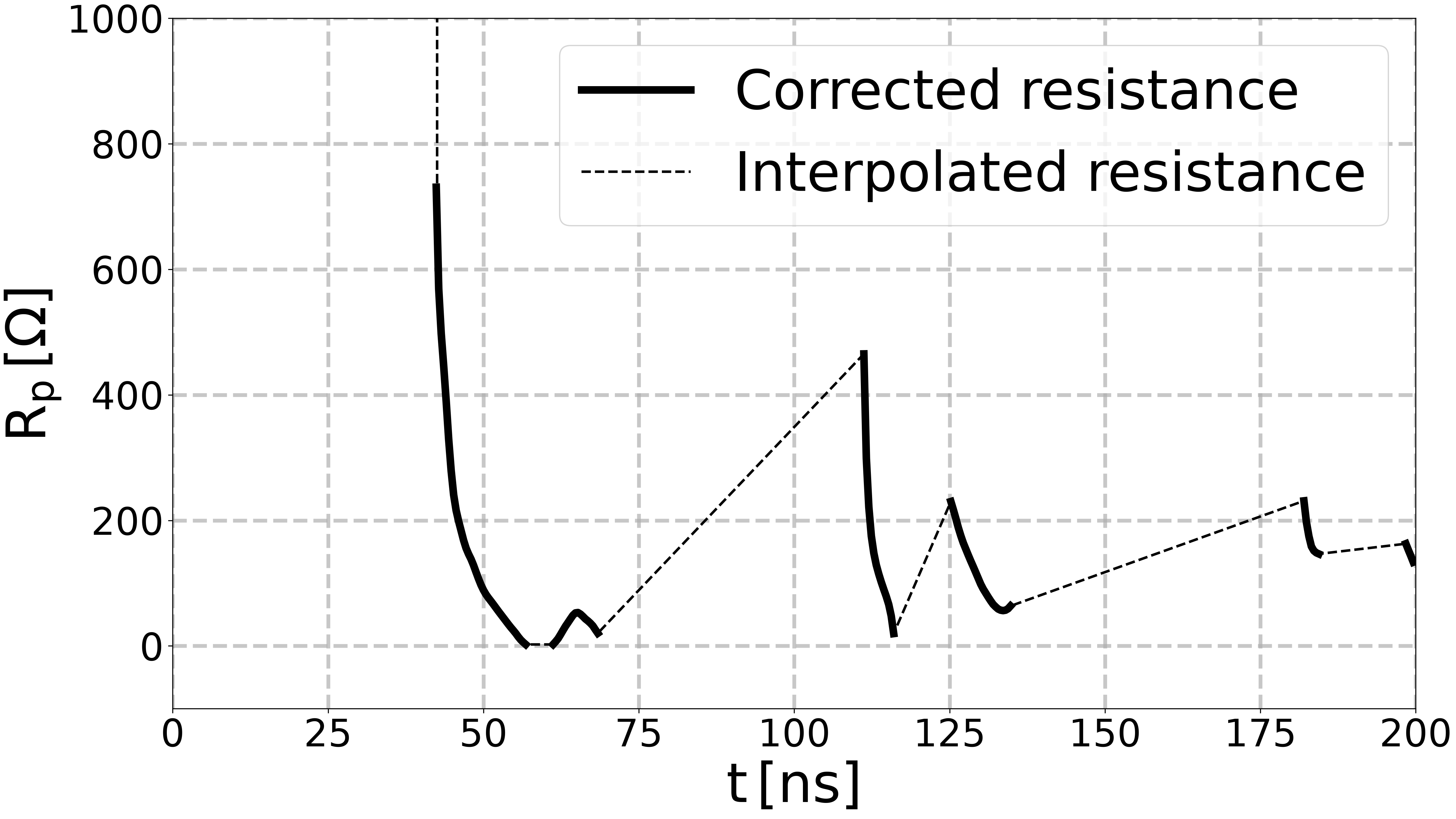
Plot the resistance vs time.#
fig, ax = expe.plot_resistance(times, show=False)
ax.set_ylim(-100, 1000)
ax.set_xlim(0, 200)
plt.show()

# Compute the plasma resistance at the times of the solution, by interpolating
# the plasma resistance computed from experimental data.
# We set `left` and `right` to `np.nan`, so that no data is extrapolated
# outside of the range of time of the experimental data.
R_p_interpolated_with_nan = np.interp(
    times,
    expe.times_corrected_with_nan,
    expe.Rp_corrected_with_nan,
    left=np.nan,
    right=np.nan,
)
Compute all the data needed to get the electron density.#
# Parameters:
# .. Atmospheric pressure
P = 1.013e5  # [Pa]
# .. Interelectrode distance (cf. [Minesi2022]_)
gap = 5e-3  # [m]
# .. Discharge radius (cf. [Minesi2022]_)
r_discharge = 0.6e-3  # [m]
# .. Discharge cross-section area.
S_discharge = np.pi * r_discharge**2  # [m^2]


@dataclass
class DataForElectronDensity:
    bolsig_data_folder: Path
    plot_color: str
    plot_linestyle: str
    plot_label: str
    temperature_K: int  # [K]
    n_gas_per_m3: float  # [m^-3]
    E_over_N_Td_bolsig: np.ndarray  # [Td]
    mu_times_N_bolsig: np.ndarray  # [1/(m*V*s)]
    mu_bolsig: np.ndarray  # [m^2/(V*s)]
    E_over_N_Td_plasma: np.ndarray  # [Td]
    mu_interpolated: np.ndarray  # [m^2/(V*s)]
    n_e_with_nan: np.ndarray  # [m^-3]
    n_e_half_with_nan: np.ndarray  # [m^-3]


# Load Bolsig+ data.
list_bolsig_files = ["2000K_Minesi2022.csv", "3000K_Minesi2022.csv"]
base_folder = get_path_to_data("Minesi2022", "cross_sections", "results")
plot_options = [
    {"color": "red", "linestyle": "-", "label": "2000 K"},
    {"color": "blue", "linestyle": "-", "label": "3000 K"},
]

all_data: list[DataForElectronDensity] = []

for file_name, plot_option in zip(list_bolsig_files, plot_options):
    data_folder = base_folder / file_name

    # Load Bolsig+ data.
    bolsig_data = np.loadtxt(data_folder, delimiter=",", skiprows=1)
    # .. Reduced electric field in Townsend.
    E_over_N_Td_bolsig = bolsig_data[:, 0]  # [Td]
    # .. Electron mobility * gas density in SI units.
    mu_times_N_bolsig = bolsig_data[:, 1]  # [1/(m*V*s)]

    # Compute electron mobility in SI units.
    # .. First, get the temperature from the file name.
    T = int(file_name.split("K")[0])  # [K]
    # .. Then, compute the gas density, assuming ideal gas behavior.
    n_gas = P / (k_b * T)  # [m^-3]
    # .. Finally, compute the mobility.
    mu_bolsig = mu_times_N_bolsig / n_gas  # [m^2/(V*s)]

    # The electron mobility is against the reduced electric field.
    # So now, we interpolate the mobility at the reduced electric field in
    # the plasma.
    # .. First, compute the electric field in the plasma.
    #    It is assumed to be uniform, and computed from the plasma voltage
    #    divided by the gap. It depends on time.
    abs_E_plasma = np.abs(plasma_voltage) / gap  # [V/m], absolute
    # .. Then, compute the reduced electric field in the plasma.
    E_over_N_Td_plasma = abs_E_plasma / n_gas * 1e21  # [Td]
    # .. Finally, interpolate the mobility at the reduced electric field in the
    #    plasma, so that it depends on time.
    #    We set `left` and `right` to `np.nan`, so that no data is extrapolated
    #    outside of the range of reduced electric field computed with Bolsig+.
    mu_interpolated = np.interp(
        E_over_N_Td_plasma,
        E_over_N_Td_bolsig,
        mu_bolsig,
        left=np.nan,
        right=np.nan,
    )

    # Finally, we can compute the electron density vs time, using the plasma
    # resistance and the mobility.
    n_e_with_nan = (
        gap  # [m]
        / S_discharge  # [m^2]
        / e  # [C] = [A*s]
        / mu_interpolated  # [m^2/(V*s)]
        / R_p_interpolated_with_nan  # [Ohm] = [V/A]
    )  # [m^-3]
    # We can also compute the density, with discharge radius divided by 2.
    # Since the density is inversely proportional to the cross-section area,
    # hich is proportional to the radius squared, it is multiplied by 4.
    n_e_half_with_nan = n_e_with_nan * 4  # [m^-3]

    data = DataForElectronDensity(
        bolsig_data_folder=data_folder,
        plot_color=plot_option["color"],
        plot_linestyle=plot_option["linestyle"],
        plot_label=plot_option["label"],
        temperature_K=T,
        n_gas_per_m3=n_gas,
        E_over_N_Td_bolsig=E_over_N_Td_bolsig,
        mu_times_N_bolsig=mu_times_N_bolsig,
        mu_bolsig=mu_bolsig,
        E_over_N_Td_plasma=E_over_N_Td_plasma,
        mu_interpolated=mu_interpolated,
        n_e_with_nan=n_e_with_nan,
        n_e_half_with_nan=n_e_half_with_nan,
    )
    all_data.append(data)
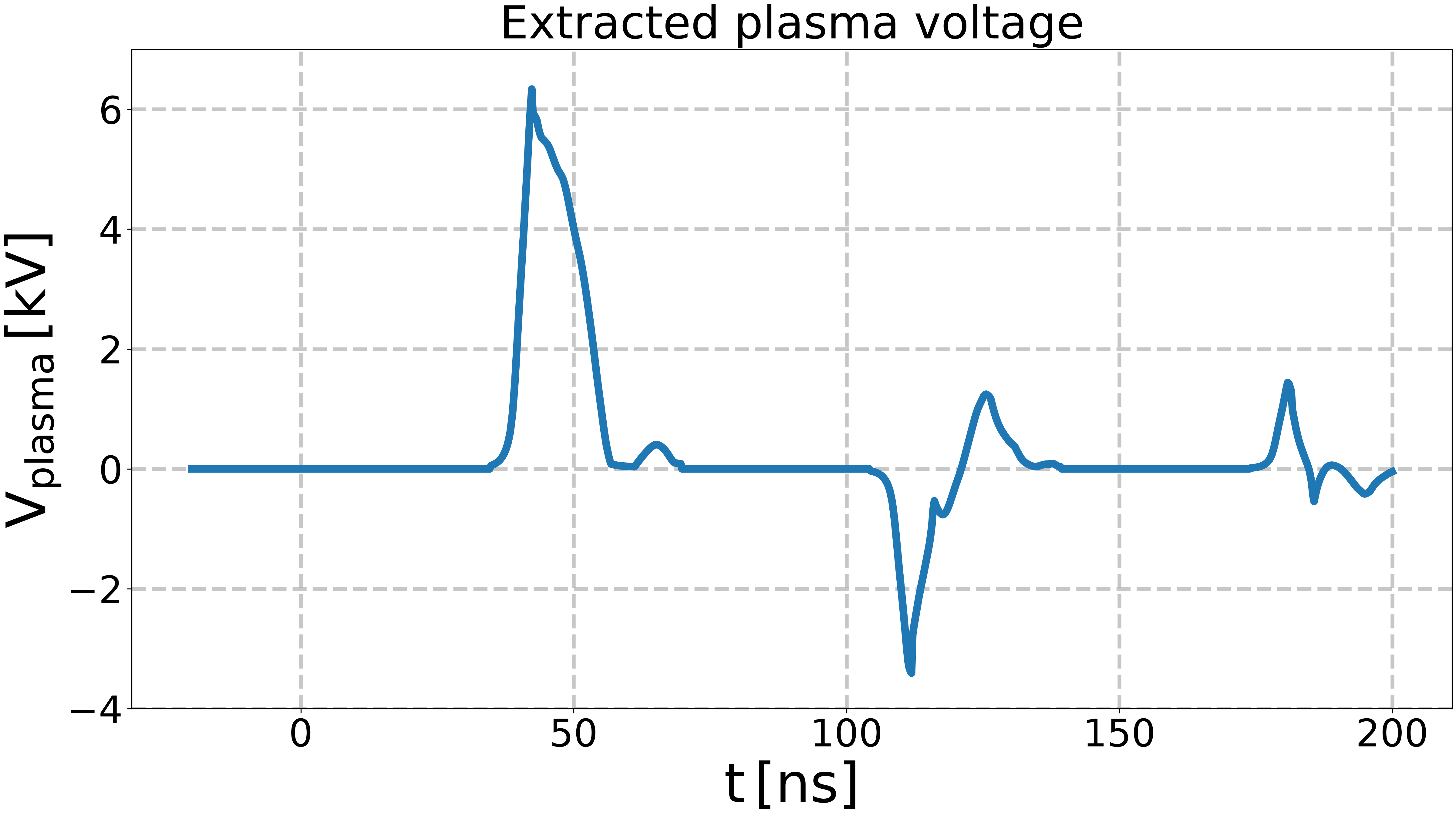
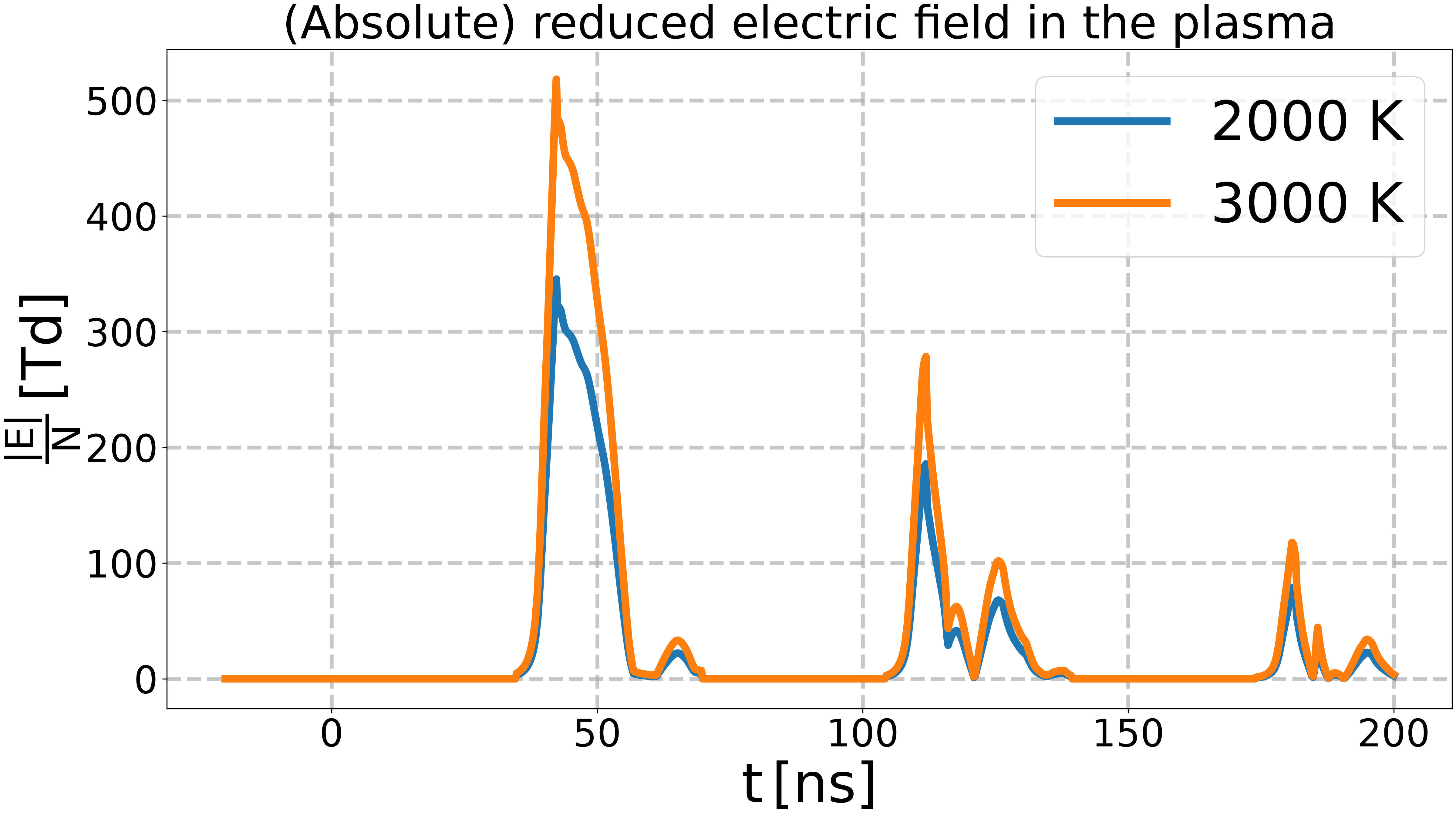
Plot reduced electric field in the plasma.#
# Plot the plasma voltage.
fig, ax = plt.subplots()
ax.plot(times * 1e9, plasma_voltage * 1e-3)
ax.set_xlabel(r"$\mathregular{t \, [ns]}$")
ax.set_ylabel(r"$\mathregular{V_{plasma} \, [kV]}$")
ax.set_title("Extracted plasma voltage")
ax.set_ylim(-4, 7)
plt.show()

# Plot the reduced electric field.
fig, ax = plt.subplots()
for data in all_data:
    ax.plot(times * 1e9, data.E_over_N_Td_plasma, label=data.plot_label)

ax.set_xlabel(r"$\mathregular{t \, [ns]}$")
ax.set_ylabel(r"$\mathregular{\frac{|E|}{N} \, [Td]}$")
ax.set_title("(Absolute) reduced electric field in the plasma")
ax.legend()
plt.show()
Plot mobility * N vs reduced electric field from Bolsig+.#
fig, ax = plt.subplots()
for data in all_data:
    ax.plot(
        data.E_over_N_Td_bolsig,
        data.mu_times_N_bolsig,
        label=data.plot_label,
        color=data.plot_color,
        linestyle=data.plot_linestyle,
    )
ax.set_title("Mobility * N from Bolsig+")
ax.set_xlabel(r"$\mathregular{E/N \, [Td]}$")
ax.set_ylabel(r"$\mathregular{\mu_e \cdot N \, [1/(m \cdot V \cdot s)]}$")
ax.set_xscale("log")
ax.legend(fontsize=20)
<matplotlib.legend.Legend object at 0x7f5d30605f70>
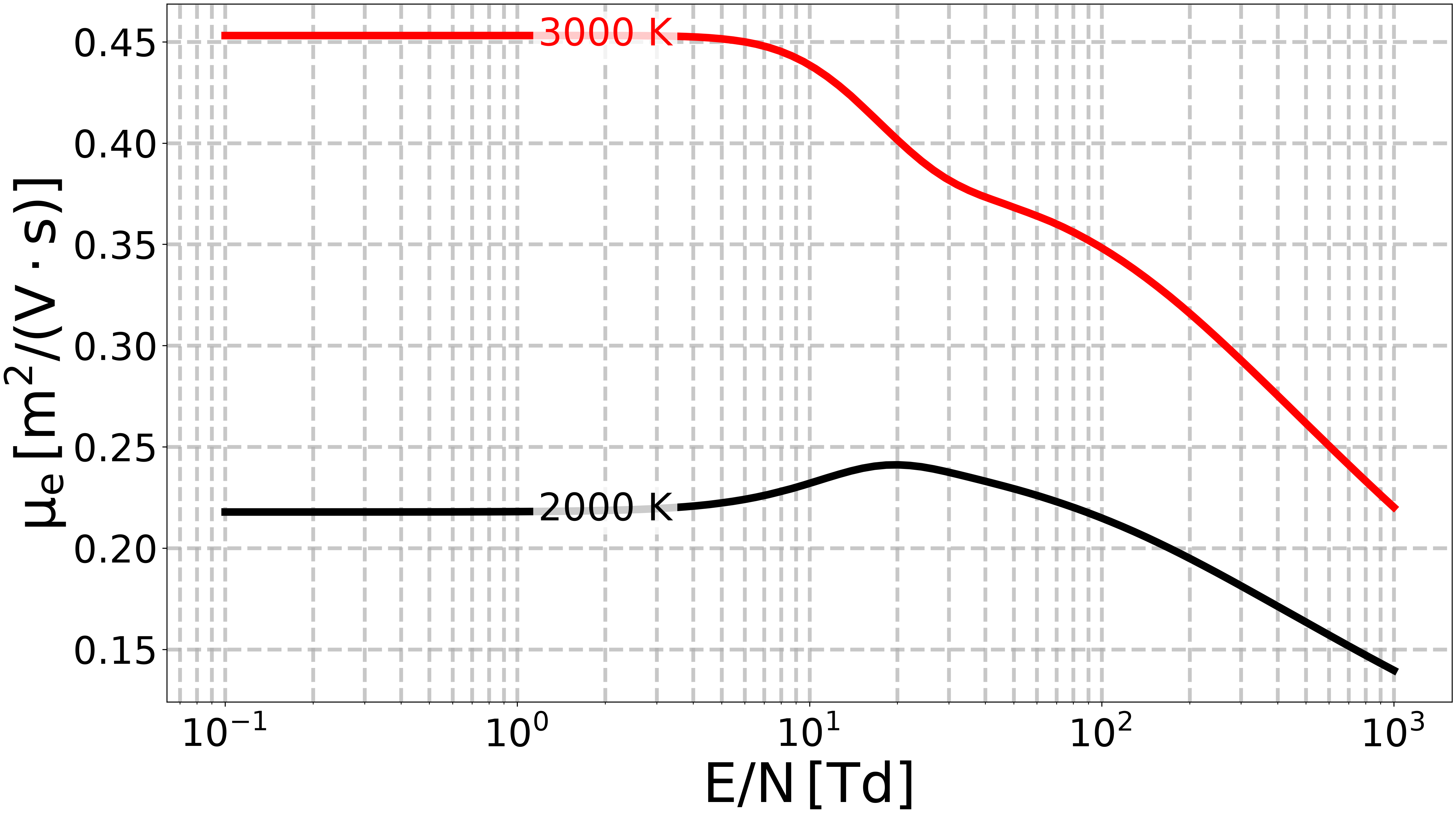
Plot mobility vs reduced electric field from Bolsig+.#
set_mpl_style(nb_columns=1)
fig, ax = plt.subplots()
colors = ["black", "red"]
x_pos_text = 2  # [Td]
for i, data in enumerate(all_data):
    ax.plot(
        data.E_over_N_Td_bolsig,
        data.mu_bolsig,
        label=data.plot_label,
        color=colors[i],
        linestyle=data.plot_linestyle,
    )
    idx_closest = np.argmin(np.abs(data.E_over_N_Td_bolsig - x_pos_text))
    ax.text(
        x_pos_text,
        data.mu_bolsig[idx_closest],
        s=data.plot_label,
        color=colors[i],
        bbox=dict(facecolor="white", alpha=0.8, edgecolor="none"),
        ha="center",
        va="center",
    )
ax.set_xlabel(r"$\mathregular{E/N \, [Td]}$")
ax.set_ylabel(r"$\mathregular{\mu_e \, [m^2/(V \cdot s)]}$")
ax.set_xscale("log")

plt.show()
# Save the figure.
fig.savefig(
    get_path_to_data(
        "article_figures",
        "Minesi2022_mobility_vs_EoverN.svg",
        force_return=True,
    )
)
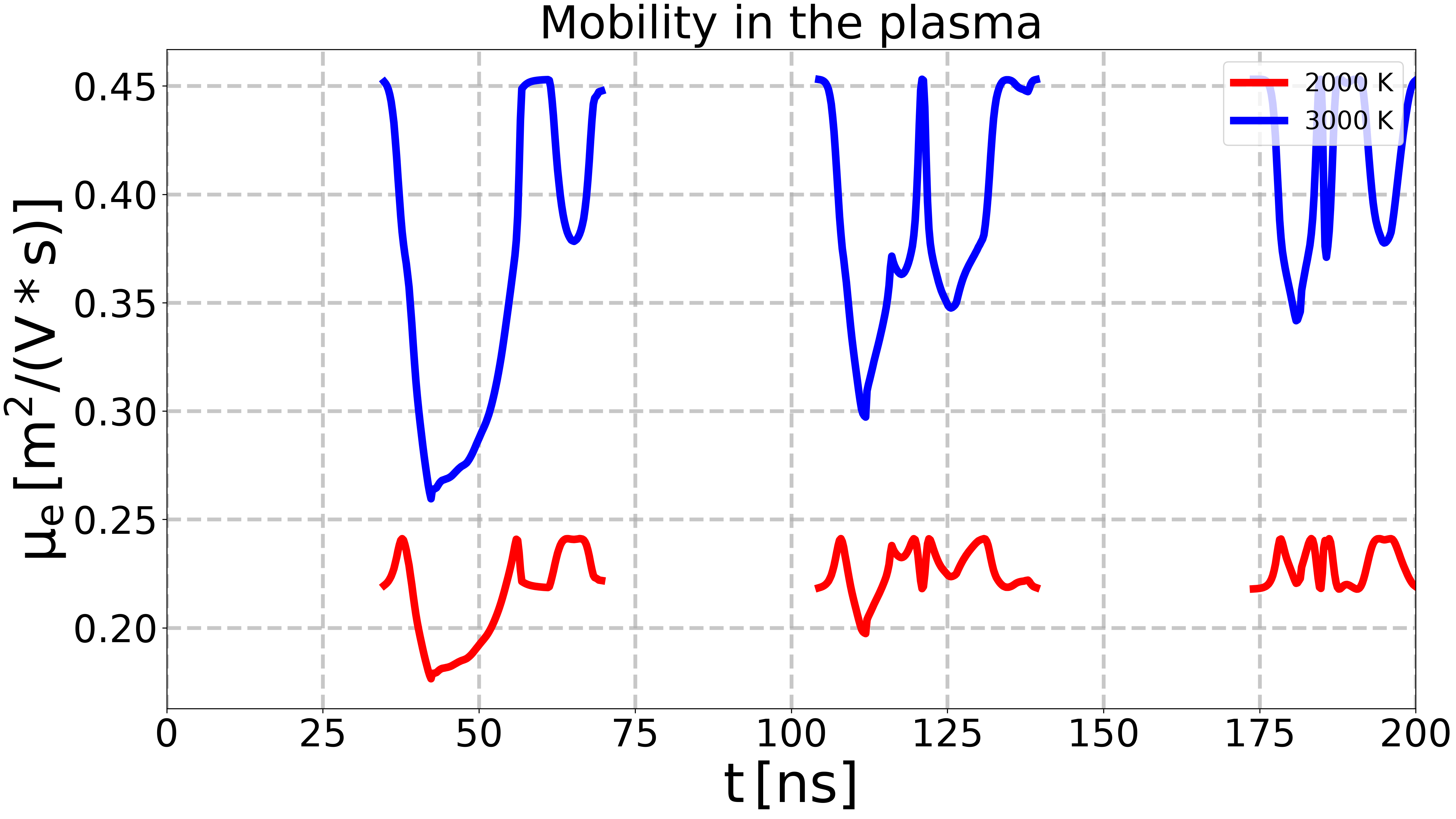
Plot the mobility vs time.#
# Plot the mobility vs time.
fig, ax = plt.subplots()
for data in all_data:
    ax.plot(
        times * 1e9,
        data.mu_interpolated,
        label=data.plot_label,
        color=data.plot_color,
        linestyle=data.plot_linestyle,
    )
ax.set_xlabel(r"$\mathregular{t \, [ns]}$")
ax.set_ylabel(r"$\mathregular{\mu_e \, [m^2/(V*s)]}$")
ax.set_title("Mobility in the plasma")
ax.legend(fontsize=20)
ax.set_xlim(0, 200)
plt.show()
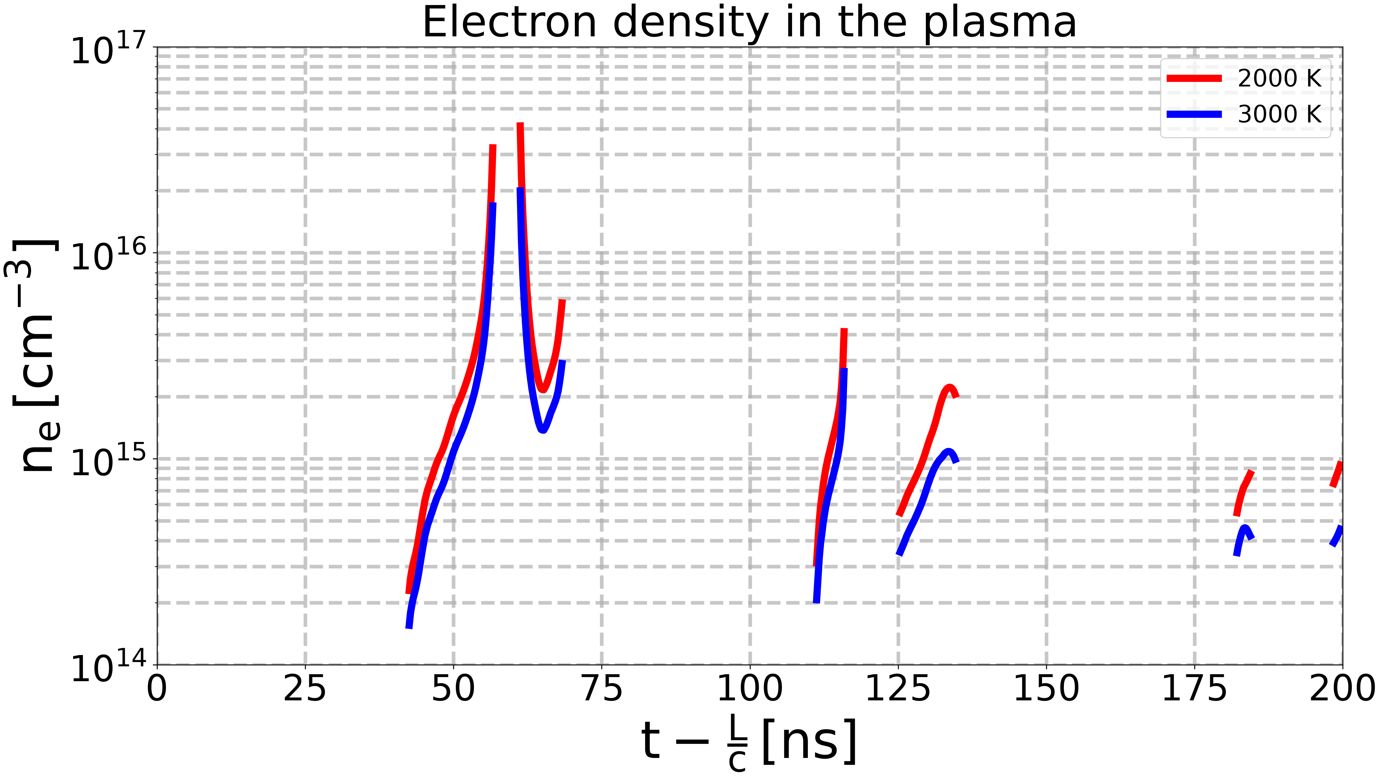
Plot the electron density vs time.#
# Plot electron density vs time.
fig, ax = plt.subplots()
for data in all_data:
    ax.plot(
        times * 1e9,
        data.n_e_with_nan * 1e-6,
        label=data.plot_label,
        color=data.plot_color,
        linestyle=data.plot_linestyle,
    )
ax.set_xlabel(r"$\mathregular{t - \frac{L}{c} \, [ns]}$")
ax.set_ylabel(r"$\mathregular{n_e \, [cm^{-3}]}$")
ax.set_title("Electron density in the plasma")
ax.set_yscale("log")
ax.legend(fontsize=20)
ax.set_xlim(0, 200)
ax.set_ylim(1e14, 1e17)
plt.show()
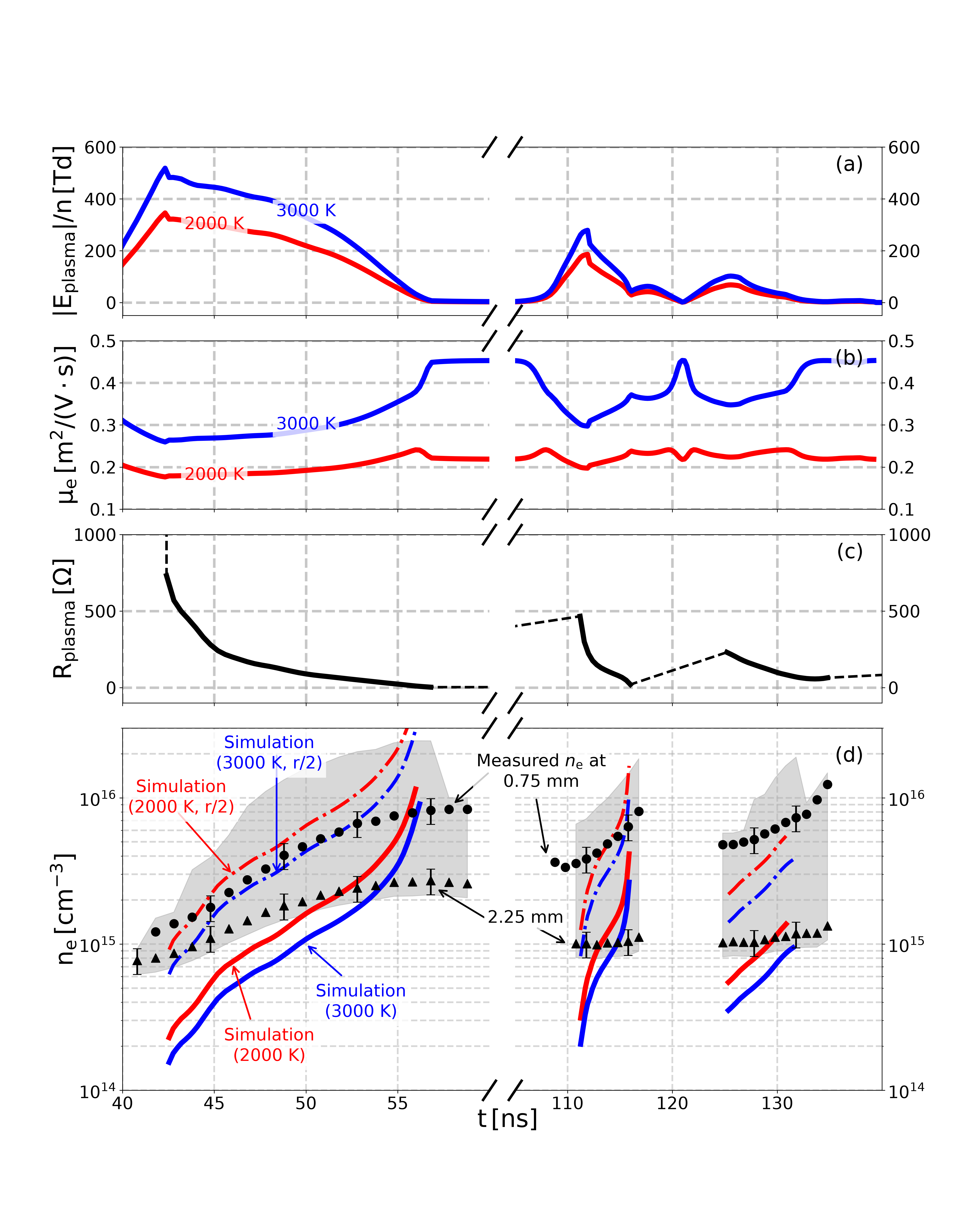
Plot the electron density vs time, with experimental data from measurements.#
set_mpl_style(nb_columns=2)

# Create the figure.
fig = plt.figure(layout="none", figsize=(16, 20))
# Add a grid of subplots to the figure:
# - First row: electric field vs time
# - Second row: mobility vs time
# - Third row: plasma resistance vs time
# - Fourth and fifth rows (merged): electron density vs time,
#   with experimental data from OES measurements.
# The two columns are for the same data, but with different y-axis limits.
gs = fig.add_gridspec(
    nrows=5,
    ncols=2,
    hspace=0.15,
    wspace=0.07,
)
ax1_E = fig.add_subplot(gs[0, 0])
ax2_E = fig.add_subplot(gs[0, 1])
ax1_mu = fig.add_subplot(gs[1, 0])
ax2_mu = fig.add_subplot(gs[1, 1])
ax1_R = fig.add_subplot(gs[2, 0])
ax2_R = fig.add_subplot(gs[2, 1])
ax1_ne = fig.add_subplot(gs[-2:, 0])
ax2_ne = fig.add_subplot(gs[-2:, 1])

# Define annotation kwargs for later use.
kwargs_annotation = dict(
    horizontalalignment="center",
    verticalalignment="center",
    fontsize=20,
    zorder=4,
    bbox=dict(facecolor="white", alpha=0.8, edgecolor="none"),
)

# Load experimental data of electron density from OES measurements.
oes_data = np.genfromtxt(
    get_path_to_data("Minesi2022", "fig7_ne_vs_time.dat"),
    delimiter="\t",
    skip_header=3,
    skip_footer=3,
)
# .. Time.
time_ns = oes_data[:, 0]  # [ns]
time_ns += L / c * 1e9  # Shift time to account for propagation delay.
time_ns += 5  # Shift time to match OES measurements with electrical ones.
# .. Electron densities.
ne_4_75mm = oes_data[:, 1]  # [cm^-3]
ne_4_25mm = oes_data[:, 2]  # [cm^-3]
ne_2_25mm = oes_data[:, 3]  # [cm^-3]
ne_0_75mm = oes_data[:, 4]  # [cm^-3]
ne_0_25mm = oes_data[:, 5]  # [cm^-3]
# Uncertainties on electron densities.
u_ne_4_75mm = oes_data[:, 6]  # [cm^-3]
u_ne_4_25mm = oes_data[:, 7]  # [cm^-3]
u_ne_2_25mm = oes_data[:, 8]  # [cm^-3]
u_ne_0_75mm = oes_data[:, 9]  # [cm^-3]
u_ne_0_25mm = oes_data[:, 10]  # [cm^-3]

# Plot experimental data from OES measurements, using the same markers/colors
# as in [Minesi2022]_ Figure 7.
ne_s = [ne_4_75mm, ne_4_25mm, ne_2_25mm, ne_0_75mm, ne_0_25mm]
u_ne_s = [u_ne_4_75mm, u_ne_4_25mm, u_ne_2_25mm, u_ne_0_75mm, u_ne_0_25mm]
labels = ["4.75 mm", "4.25 mm", "2.25 mm", "0.75 mm", "0.25 mm"]
markers = ["D", "v", "^", "o", "s"]
colors = ["m", "g", "b", "r", "k"]
xy_labels = [(105, 1.2e16), (105, 3e15), (105, 1e15), (105, 7e15), (105, 2e16)]
# for ne, u_ne, label, marker, color, xy in zip(
#     ne_s, u_ne_s, labels, markers, colors, xy_labels
# ):
#     for ax in (ax1_ne, ax2_ne):
#         # Plot experimental electron density without error bars.
#         ax.scatter(
#             time_ns,
#             ne,
#             s=100,
#             marker=marker,
#             color=color,
#             zorder=3,
#         )
#         # Plot experimental electron density with error bars, every 4 points.
#         ax.errorbar(
#             time_ns[::4],
#             ne[::4],
#             yerr=u_ne[::4],
#             fmt=marker,
#             markersize=10,
#             color=color,
#             ecolor=color,
#             elinewidth=2,
#             capsize=5,  # Size of the error bar caps
#             zorder=3,
#         )
#     # .. Annotate the electron density plot (experimental).
#     ax2_ne.text(
#         *xy,
#         s=label,
#         color=color,
#         **kwargs_annotation,  # type: ignore
#     )

# Alternate graph: only the measured electron density at 0.75 mm is shown.
# A grey area is added, covering all the measured electron densities.
for ax in (ax1_ne, ax2_ne):
    # .. Grey area.
    ax.fill_between(
        time_ns,
        ne_2_25mm - u_ne_2_25mm,
        np.nanmax(ne_s, axis=0) + np.nanmax(u_ne_s, axis=0),
        color="grey",
        alpha=0.3,
        zorder=1,
    )
    # .. Measured electron density at 0.75 mm.
    ax.scatter(
        time_ns,
        ne_0_75mm,
        s=100,
        marker="o",
        color="k",
        zorder=3,
    )
    ax.errorbar(
        time_ns[::4],
        ne_0_75mm[::4],
        yerr=u_ne_0_75mm[::4],
        fmt="o",
        markersize=10,
        color="k",
        ecolor="k",
        elinewidth=2,
        capsize=5,  # Size of the error bar caps
        zorder=3,
    )

    # .. Also plot electron density at 2.25 mm.
    ax.scatter(
        time_ns,
        ne_2_25mm,
        s=100,
        marker="^",
        color="k",
        zorder=3,
    )
    ax.errorbar(
        time_ns[::4],
        ne_2_25mm[::4],
        yerr=u_ne_2_25mm[::4],
        fmt="^",
        markersize=10,
        color="k",
        ecolor="k",
        elinewidth=2,
        capsize=5,  # Size of the error bar caps
        zorder=3,
    )


# .. Annotate the electron density plot (experimental).
ax2_ne.text(
    x=107.5,
    y=1.5e16,
    s=r"Measured $n_\text{e}$ at" + "\n0.75 mm",
    color="k",
    **kwargs_annotation,  # type: ignore
)
# .. Add two arrows.
ax2_ne.annotate(
    "",
    xy=(108, 4e15),
    xytext=(107, 1e16),
    arrowprops=dict(arrowstyle="->", color="k", lw=2),
)
ax1_ne.annotate(
    "",
    xy=(58, 9e15),
    xytext=(60, 1.5e16),
    arrowprops=dict(arrowstyle="->", color="k", lw=2),
)

# .. Annotate for 2.25 mm.
ax2_ne.text(
    x=106,
    y=1.5e15,
    s="2.25 mm",
    color="k",
    **kwargs_annotation,  # type: ignore
)
# .. Add two arrows.
ax2_ne.annotate(
    "",
    xy=(110, 1e15),
    xytext=(107, 1.3e15),
    arrowprops=dict(arrowstyle="->", color="k", lw=2),
)
ax1_ne.annotate(
    "",
    xy=(57.1, 2.4e15),
    xytext=(59.8, 1.5e15),
    arrowprops=dict(arrowstyle="->", color="k", lw=2),
)


# Plot numerical results of electron density.
for ax in (ax1_ne, ax2_ne):
    for data in all_data:
        # Mask for the electric field.
        mask = data.E_over_N_Td_plasma > 20  # [Td]

        ne_per_cm3 = data.n_e_with_nan * 1e-6  # [cm^-3]
        ne_per_cm3[~mask] = np.nan

        # Plot electron density (normal radius).
        ax.plot(
            times * 1e9,
            ne_per_cm3,
            zorder=2,
            color=data.plot_color,
            linestyle=data.plot_linestyle,
        )

        # Also plot the results with half the discharge radius.
        ne_half_per_cm3 = data.n_e_half_with_nan * 1e-6  # [cm^-3]
        ne_half_per_cm3[~mask] = np.nan

        ax.plot(
            times * 1e9,
            ne_half_per_cm3,
            color=data.plot_color,
            linestyle="-.",
            linewidth=4,
        )

# Plot plasma resistance.
for ax in (ax1_R, ax2_R):
    ax.plot(
        expe.times_corrected * 1e9,
        expe.Rp_corrected * 1e0,
        color="k",
        ls="--",
        lw=3,
    )
    ax.plot(
        expe.times_corrected_with_nan * 1e9,
        expe.Rp_corrected_with_nan,
        color="black",
    )

# Plot mobility.
for ax in (ax1_mu, ax2_mu):
    for data in all_data:
        ax.plot(
            times * 1e9,
            data.mu_interpolated,
            label=data.plot_label,
            color=data.plot_color,
            linestyle=data.plot_linestyle,
        )

# Plot electric field.
for ax in (ax1_E, ax2_E):
    for data in all_data:
        ax.plot(
            times * 1e9,
            data.E_over_N_Td_plasma,
            label=f"E/N ({data.temperature_K} K)",
            color=data.plot_color,
        )


# Plot settings.
for ax1, ax2 in [
    (ax1_ne, ax2_ne),
    (ax1_R, ax2_R),
    (ax1_mu, ax2_mu),
    (ax1_E, ax2_E),
]:
    # .. Hide the spines between ax and ax2.
    ax1.spines["right"].set_visible(False)
    ax2.spines["left"].set_visible(False)
    ax1.yaxis.tick_left()
    ax2.yaxis.tick_right()

    # .. Add diagonal lines to indicate the break in the x-axis.
    d = 1.5  # Proportion of vertical to horizontal extent of the slanted line.
    kwargs = dict(
        marker=[(-1, -d), (1, d)],
        markersize=25,
        linestyle="none",
        color="k",
        mec="k",
        mew=3,
        clip_on=False,
    )
    ax1.plot([1, 1], [0, 1], transform=ax1.transAxes, **kwargs)  # type: ignore
    ax2.plot([0, 0], [0, 1], transform=ax2.transAxes, **kwargs)  # type: ignore

    # .. Change x-limits.
    ax1.set_xlim(40, 60)
    ax2.set_xlim(105, 140)

    # .. Remove x-ticks for all plots.
    ax1.set_xticks([40, 45, 50, 55])
    ax2.set_xticks([110, 120, 130])
    ax1.set_xticklabels([])
    ax2.set_xticklabels([])

    # .. Place the y-axis labels in the middle of the plots.
    ax1.yaxis.set_label_coords(-0.12, 0.5)

# .. Set x-ticks, only for the bottom plots.
ax1_ne.set_xticks([40, 45, 50, 55])
ax1_ne.set_xticklabels(["40", "45", "50", "55"])
ax2_ne.set_xticks([110, 120, 130])
ax2_ne.set_xticklabels(["110", "120", "130"])

# .. Change y-scale and y-limits
for ax in (ax1_ne, ax2_ne):
    ax.set_yscale("log")
    ax.set_ylim(1e14, 3e16)
for ax in (ax1_R, ax2_R):
    ax.set_ylim(-100, 1000)
for ax in (ax1_mu, ax2_mu):
    ax.set_ylim(0.1, 0.5)
for ax in (ax1_E, ax2_E):
    ax.set_ylim(-50, 600)

# .. Add labels.
ax1_ne.set_xlabel(r"$\mathregular{t \, [ns]}$")
ax1_ne.set_ylabel(r"$\mathregular{n_e \, [cm^{-3}]}$")
ax1_R.set_ylabel(r"$\mathregular{R_{plasma} \, [\Omega]}$")
ax1_mu.set_ylabel(r"$\mathregular{\mu_e \, [m^2/(V \cdot s)]}$")
ax1_E.set_ylabel(r"$\mathregular{|E_{plasma}|/n \, [Td]}$")

# .. Change position of x-axis label.
ax1_ne.xaxis.set_label_coords(1.05, -0.05)
ax1_R.xaxis.set_label_coords(1.05, -0.05)

# .. Annotate the electron density plot (numerical).
ax1_ne.text(
    48,
    2e14,
    "Simulation\n(2000 K)",
    color="red",
    **kwargs_annotation,  # type: ignore
)
ax1_ne.text(
    53,
    4e14,
    "Simulation\n(3000 K)",
    color="blue",
    **kwargs_annotation,  # type: ignore
)
# Create arrows for the annotations.
ax1_ne.annotate(
    "",
    xy=(46, 7.4e14),
    xytext=(47, 3e14),
    arrowprops=dict(color="red", arrowstyle="->", lw=2),
)
ax1_ne.annotate(
    "",
    xy=(50, 1e15),
    xytext=(52, 6e14),
    arrowprops=dict(color="blue", arrowstyle="->", lw=2),
)

ax1_ne.text(
    43.2,
    1e16,
    "Simulation\n(2000 K, r/2)",
    color="red",
    **kwargs_annotation,  # type: ignore
)
ax1_ne.text(
    48,
    2e16,
    "Simulation\n(3000 K, r/2)",
    color="blue",
    **kwargs_annotation,  # type: ignore
)
# Create arrows for the (r/2) annotations.
ax1_ne.annotate(
    "",
    xy=(46, 3e15),
    xytext=(43, 8e15),
    arrowprops=dict(color="red", arrowstyle="->", lw=2),
)
ax1_ne.annotate(
    "",
    xy=(48.4, 3e15),
    xytext=(48.4, 2e16),
    arrowprops=dict(color="blue", arrowstyle="->", lw=2),
)

# .. Annotate the electric field plot.
ax1_E.text(45, 300, "2000 K", color="red", **kwargs_annotation)  # type: ignore
ax1_E.text(50, 350, "3000 K", color="blue", **kwargs_annotation)  # type: ignore

# .. Annotate the mobility plot.
ax1_mu.text(45, 0.18, "2000 K", color="red", **kwargs_annotation)  # type: ignore
ax1_mu.text(50, 0.3, "3000 K", color="blue", **kwargs_annotation)  # type: ignore

# .. Add in the upper right corner the subplot label (a), (b), ...
subplot_labels = ["(a)", "(b)", "(c)", "(d)"]
all_axes = [ax2_E, ax2_mu, ax2_R, ax2_ne]
for ax, label in zip(all_axes, subplot_labels):
    ax.text(
        0.95,
        0.95,
        label,
        transform=ax.transAxes,
        horizontalalignment="right",
        verticalalignment="top",
        fontsize=24,
        bbox=dict(facecolor="white", alpha=0.8, edgecolor="none"),
    )

# .. Adjust grid for the electron density plots.
for ax in (ax1_ne, ax2_ne):
    ax.grid(visible=True, which="both", linestyle="--", linewidth=2, alpha=0.5)

plt.show()
/home/runner/work/pyresiflex/pyresiflex/examples/article_figures/plot_get_electron_density_from_Minesi2022_experiments.py:724: RuntimeWarning: All-NaN axis encountered
  np.nanmax(ne_s, axis=0) + np.nanmax(u_ne_s, axis=0),
Save the figure.#
# Keep the layout to "none",
# so that the saved figure looks exactly like the one shown.
fig.set_layout_engine("none")


fig.savefig(
    get_path_to_data(
        "article_figures",
        "Minesi2022_comparison_electron_density.svg",
        force_return=True,
    ),
    bbox_inches="tight",
)
Total running time of the script: (0 minutes 10.599 seconds)