Reproducing [PerrinTerrin2025] experiments.

In this example, the plasma is a time-varying resistance.

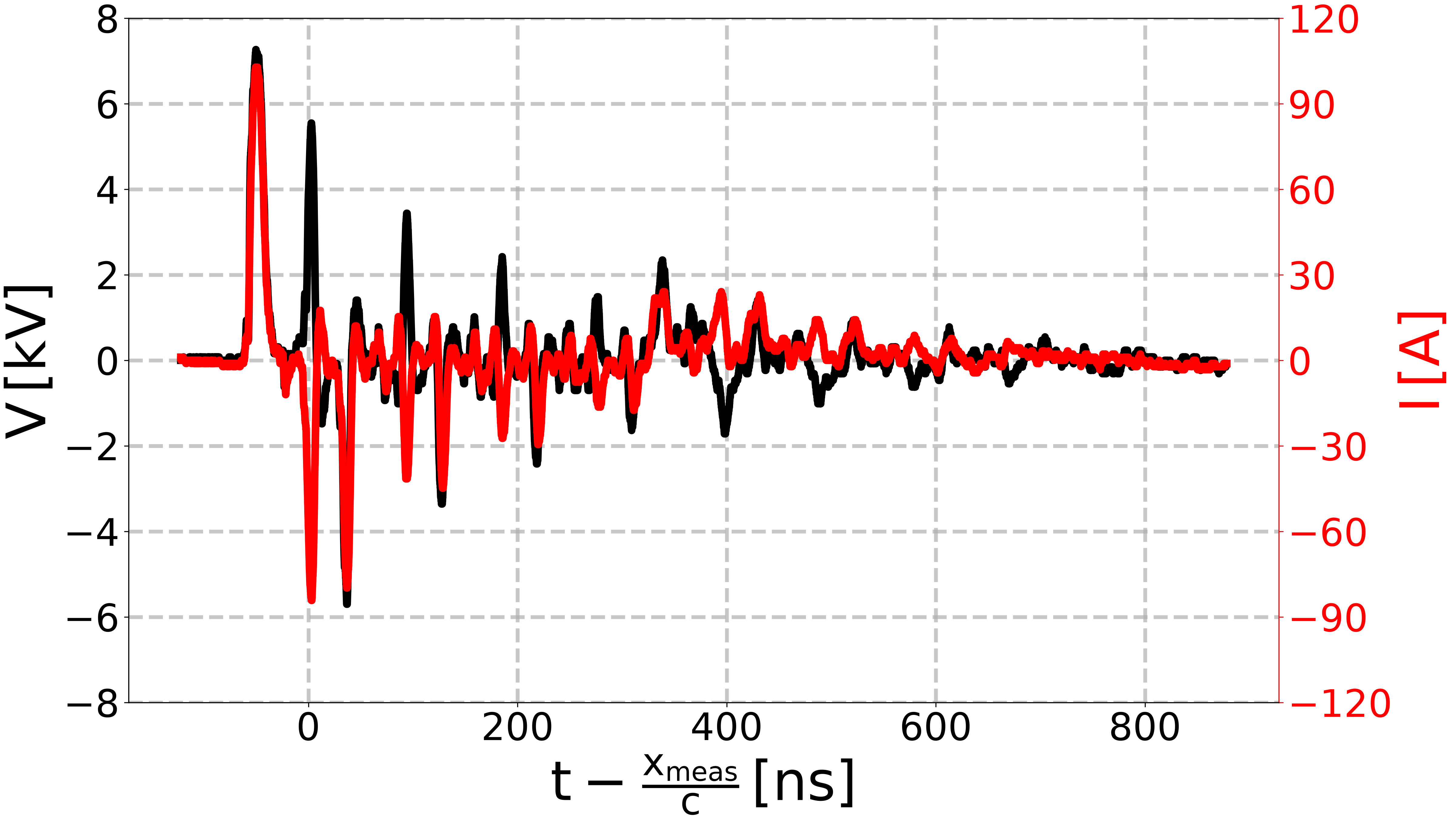
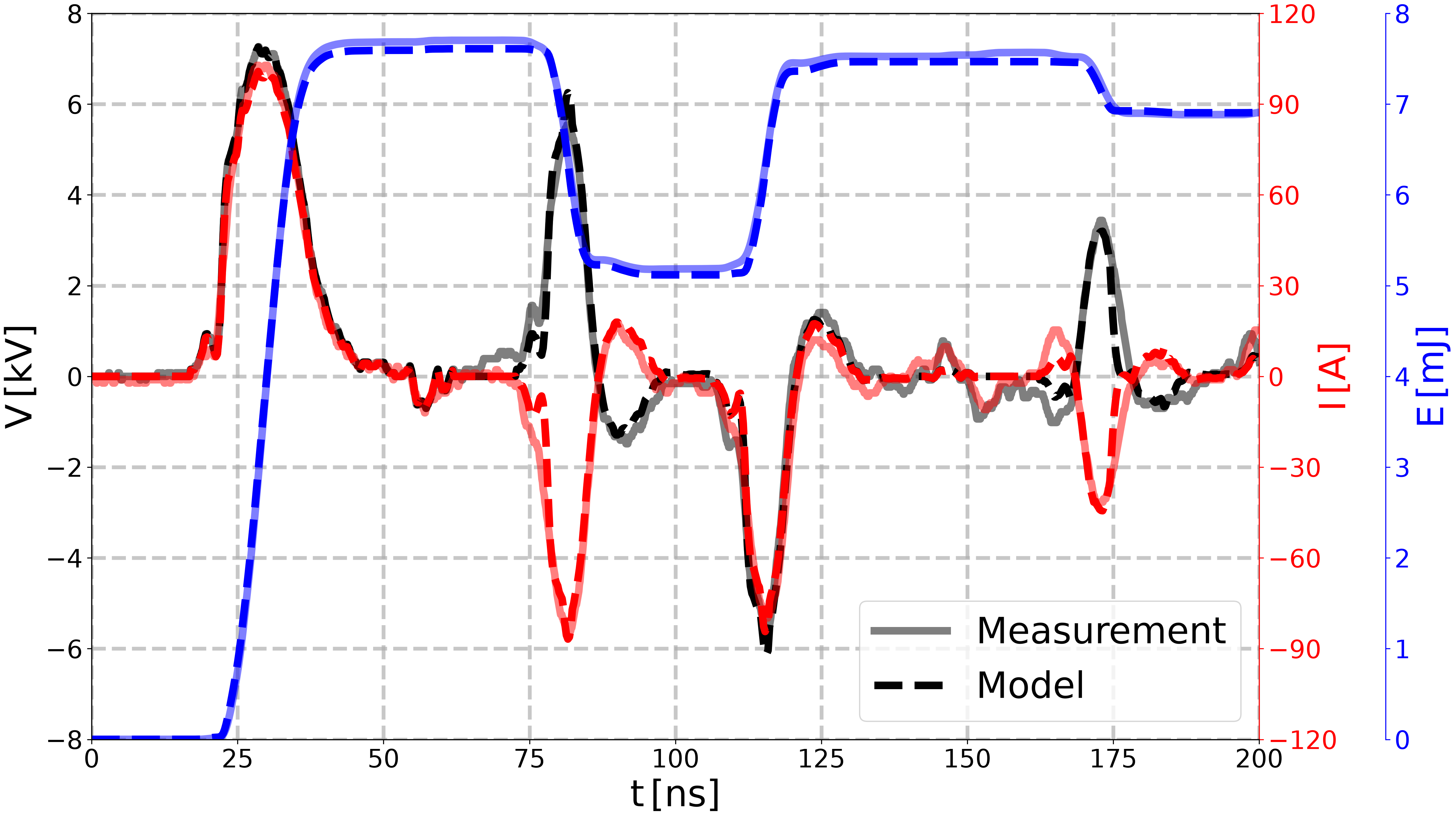
Experimental data of [PerrinTerrin2025] are used to extract the plasma resistance, and to reconstruct the voltage and current signals. Probes are located at around 3 meters from the generator, while the plasma is located at around 8 meters from the generator.

# This sets the fifth figure as the thumbnail for the example gallery.
# sphinx_gallery_thumbnail_number = 5
# This displays each image separately in the example gallery.
# sphinx_gallery_multi_image = "single"

First, we import the required libraries.

We start by importing the modules we need:

• matplotlib for drawing graphs,

• numpy for array functions,

• pyresiflex for the generator, load and transmission line.

import matplotlib.pyplot as plt
import numpy as np

from pyresiflex.cable.cable import PerfectCable
from pyresiflex.experiment.purely_resistive_experiment import (
    PurelyResistiveExperiment,
)
from pyresiflex.generator.generator_real_impedance import (
    FromMeasurementGenerator,
)
from pyresiflex.misc.plot import plot_voltage_current, set_mpl_style
from pyresiflex.misc.utils import get_path_to_data
from pyresiflex.solver.purely_resistive_solution import PurelyResistiveSolution

set_mpl_style(nb_columns=1)

Load [PerrinTerrin2025] experimental data of remote configuration.

# Load the raw data from Figure 16 of [PerrinTerrin2025]_.
file = get_path_to_data(
    "PerrinTerrin2025",
    "C1run_6_V_13kV_frep_20kHz_Pth_50kW_Qair_55p5per_alpha_40__0020_0.csv",
)
data = np.loadtxt(file, skiprows=3, delimiter=",")
times_raw = data[:, 0]  # [s]
voltages_raw = data[:, 1]  # [V]
currents_raw = data[:, 2]  # [A]

# Plot the raw data.
fig, ax_v, ax_i = plot_voltage_current(
    voltage_time=times_raw,
    voltage_value=voltages_raw,
    current_time=times_raw,
    current_value=currents_raw,
)
ax_v.set_xlabel(r"$\mathregular{t - \frac{x_{meas}}{c} \, [ns]}$")
ax_v.set_ylim(-8, 8)
ax_i.set_ylim(-120, 120)
ax_i.set_yticks([-120, -90, -60, -30, 0, 30, 60, 90, 120])

plt.show()

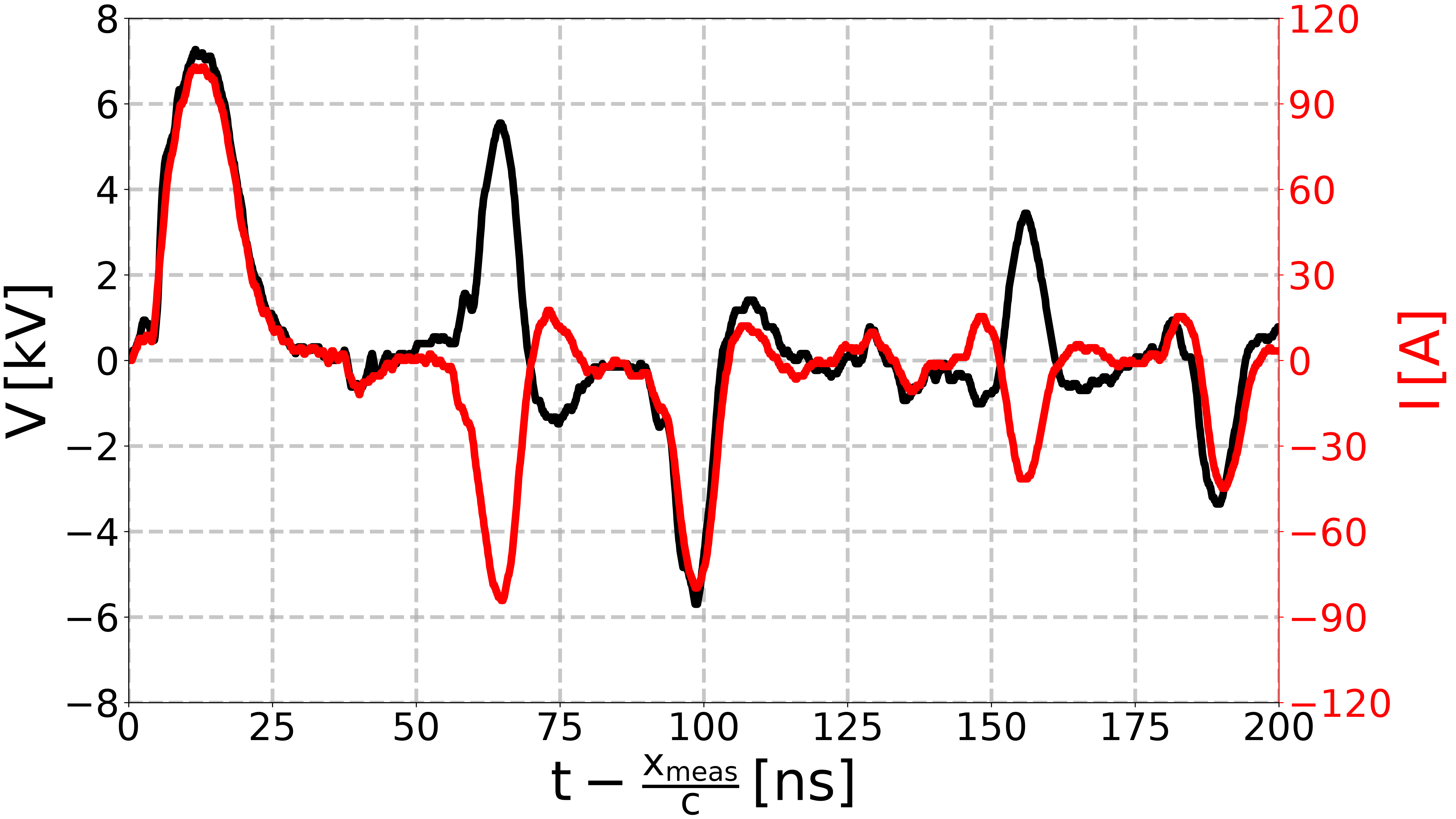
Preprocess the data.

# Define the zero at the first time the voltage reaches `threshold_voltage`.
threshold_voltage = 100  # [V]
idx_first = np.where(np.abs(voltages_raw) > threshold_voltage)[0][0]
times_raw = times_raw - times_raw[idx_first]

# Define a time window to analyze.
lower_time_window = -20e-9  # [s]
upper_time_window = 200e-9  # [s]

# Limit the time window to [lower_time_window, upper_time_window]
idx_min_wanted_time = np.where(times_raw > lower_time_window)[0][0]
idx_max_wanted_time = np.where(times_raw > upper_time_window)[0][0]

# Limit the time, voltages and currents to the wanted period.
times_expe = times_raw[idx_min_wanted_time:idx_max_wanted_time]
voltages_expe = voltages_raw[idx_min_wanted_time:idx_max_wanted_time]
currents_expe = currents_raw[idx_min_wanted_time:idx_max_wanted_time]

# Compute the energy from the voltage and current.
energies_expe = np.zeros_like(times_expe)  # [J]
for i in range(len(times_expe)):
    energies_expe[i] = np.trapezoid(
        voltages_expe[:i] * currents_expe[:i], times_expe[:i]
    )


# Plot the preprocessed data.
fig, ax_v, ax_i = plot_voltage_current(
    voltage_time=times_expe,
    voltage_value=voltages_expe,
    current_time=times_expe,
    current_value=currents_expe,
)
ax_v.set_xlabel(r"$\mathregular{t - \frac{x_{meas}}{c} \, [ns]}$")
ax_v.set_xlim(0, 200)
ax_v.set_ylim(-8, 8)
ax_i.set_ylim(-120, 120)
ax_i.set_yticks([-120, -90, -60, -30, 0, 30, 60, 90, 120])

plt.show()

# Save the figure.
fig.savefig(
    get_path_to_data(
        "article_figures",
        "PerrinTerrin2025_voltage_current_experimental_measurement.svg",
        force_return=True,
    ),
)

Transmission line parameters

# Length of the transmission line
L = 8.2  # [m]
# Measurement points = probe positions
x = 3.1  # [m]
# Here, we assume that the probes are located at the same position.
x_meas_voltage = x_meas_current = x  # [m]
# Velocity of propagation of the wave in the cable.
c = 1.83e8  # [m/s]
# Cable characteristic impedance.
Z_c = 72  # [Ohm]

cable = PerfectCable(
    L=L,
    Z_c=Z_c,
    c=c,
)

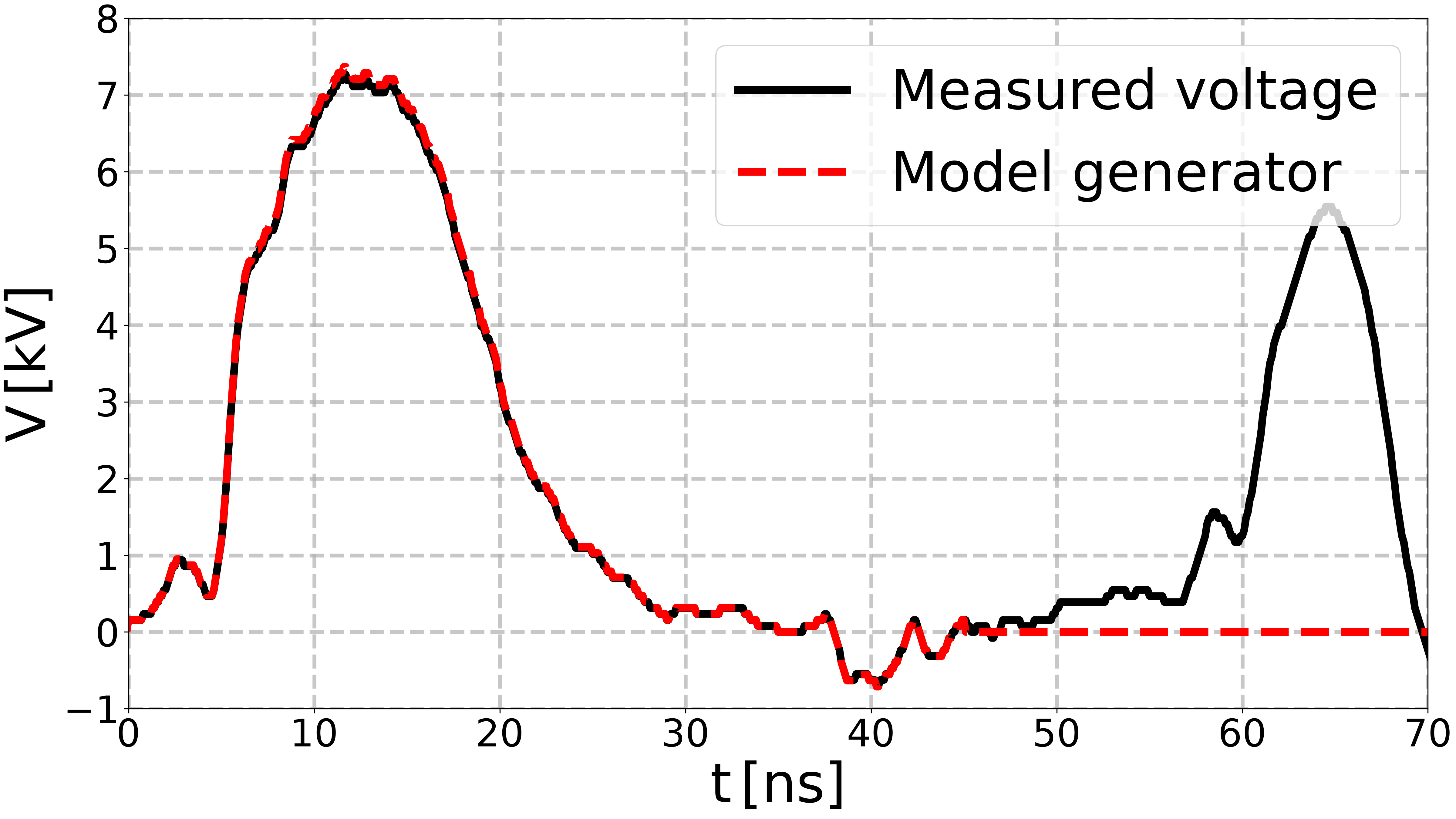
Generator parameters

# Impedance of the generator.
R_g = 1  # [Ohm]
# Attenuation coefficient.
alpha_g = Z_c / (Z_c + R_g)  # [-]
# Pulse duration.
pulse_duration = 45e-9  # [s]


def V_meas_generator(t, times, voltages):
    if t < 0:
        return 0.0
    elif t > pulse_duration:
        return 0.0
    else:
        return np.interp(t, times, voltages) / alpha_g


generator = FromMeasurementGenerator(
    R_g=R_g, V_meas=lambda t: V_meas_generator(t, times_expe, voltages_expe)
)

# Plot the voltage signal.
fig, ax = plt.subplots()

ax.plot(
    times_expe * 1e9,
    voltages_expe * 1e-3,
    color="black",
    label="Measured voltage",
)
ax.plot(
    times_expe * 1e9,
    [generator.generator_voltage(t) * 1e-3 for t in times_expe],
    "--",
    label="Model generator",
    color="red",
)
ax.set_xlabel(r"$\mathregular{t \, [ns]}$")
ax.set_ylabel(r"$\mathregular{V \, [kV]}$")
ax.set_xlim(0, 70)
ax.set_ylim(-1, 8.0)
ax.legend()
plt.show()

# Save the figure.
fig.savefig(
    get_path_to_data(
        "article_figures",
        "PerrinTerrin2025_generator_voltage_model.svg",
        force_return=True,
    ),
)

Load parameters.

expe = PurelyResistiveExperiment(
    experimental_voltage_time=times_expe,
    experimental_voltage_value=voltages_expe,
    x_meas_voltage=x_meas_voltage,
    experimental_current_time=times_expe,
    experimental_current_value=currents_expe,
    x_meas_current=x_meas_current,
    L=L,
    Z_c=Z_c,
    c=c,
    correct_time_zero=True,
)

threshold_voltage_reconstruction = 0.2 * np.max(voltages_expe)  # [V]
expe.compute_plasma_resistance_from_vmeas_and_imeas(
    times_expe,
    threshold=threshold_voltage_reconstruction,
    channel_formation_time=0.0,
)

plasma_load = expe.load_corrected

fig, ax = expe.plot_resistance(times=times_expe)
ax.set_xlim(50, 150)
ax.set_ylim(-100, 1000)
plt.show()

# Save the figure.
fig.savefig(
    get_path_to_data(
        "article_figures",
        "PerrinTerrin2025_plasma_resistance_with_time.svg",
        force_return=True,
    ),
)

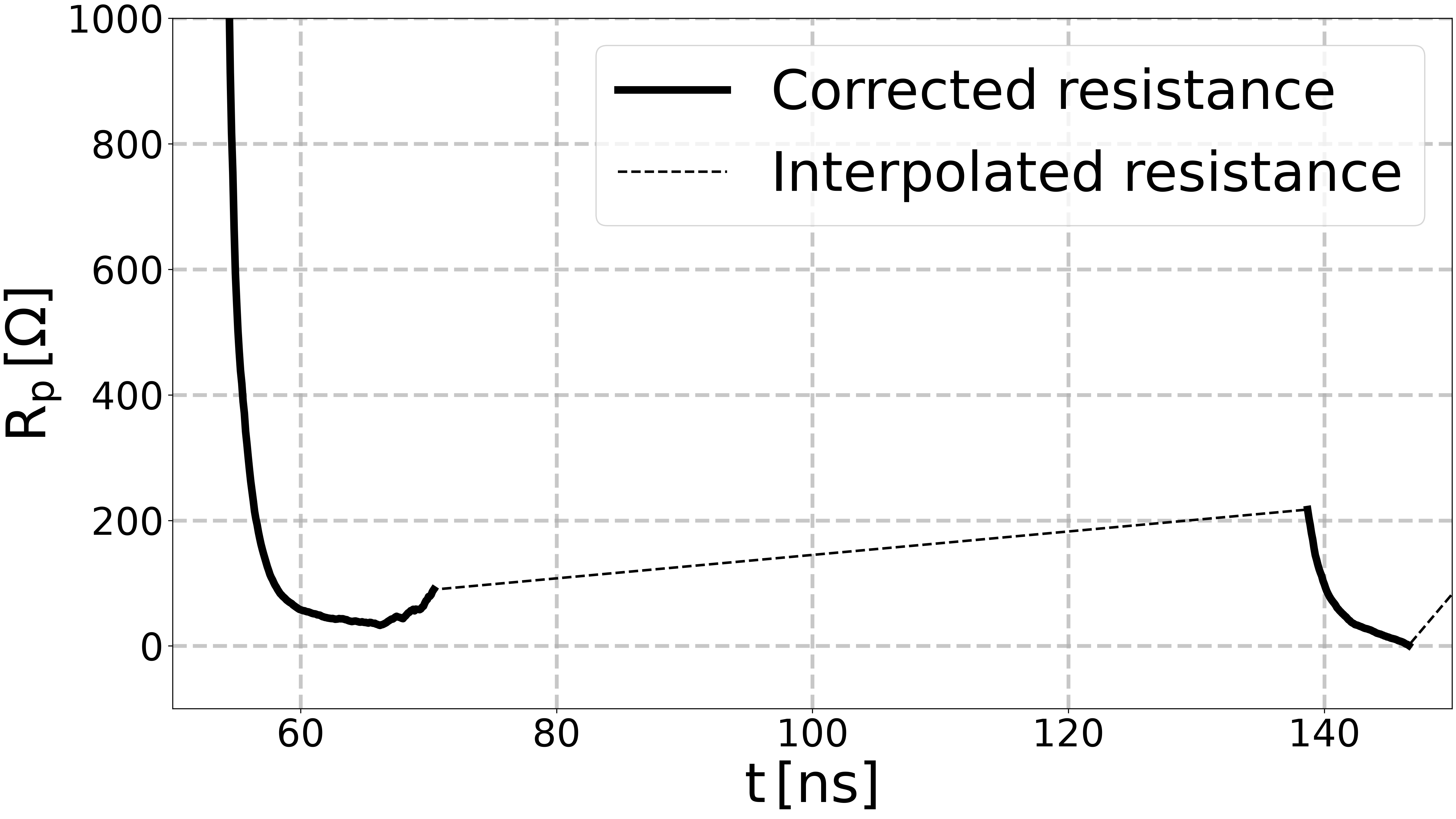
/home/runner/work/pyresiflex/pyresiflex/src/pyresiflex/experiment/purely_resistive_experiment.py:290: UserWarning: Some values in the denominator are zero, resistance cannot be computed correctly. These values are set to 1 MOhm.
  warn(

Solution object.

solution = PurelyResistiveSolution(
    generator=generator,
    load=plasma_load,
    cable=cable,
)

Compute voltage and current at a given position.

# Time vector for the simulation.
nb_steps = 1000
times = np.linspace(0, 250e-9, nb_steps)  # [s]

# Compute the voltage and current at a given position.
solution.solve(x, times)

voltages = solution.voltage  # [V]
currents = solution.current  # [A]
energies = solution.energy  # [J]
xs = solution.x  # [m]
times = solution.t  # [s]

Plot voltage, current, and energy at remote configuration.

set_mpl_style(nb_columns=2)

# Do we want to plot the current and energy?
plot_current = True
plot_energy = True
# Do we want to shift the time axis to have t - x/c?
shift_time_axis = False

if shift_time_axis:
    times_shifted = times - x / c
    times_expe_shifted = times_expe
    x_label = r"$\mathregular{t - \frac{x_{meas}}{c} \, [ns]}$"
else:
    times_shifted = times
    times_expe_shifted = times_expe + x / c
    x_label = r"$\mathregular{t \, [ns]}$"


fig, ax_v = plt.subplots()

# Plot voltage.
plot_line_v = ax_v.plot(
    times_shifted * 1e9,
    voltages * 1e-3,
    color="k",
    ls="--",
    label="Voltage (computed)",
)
plot_line_v_measured = ax_v.plot(
    times_expe_shifted * 1e9,
    voltages_expe * 1e-3,
    color="k",
    label="Voltage (experimental)",
    alpha=0.5,
)
# .. Plot options for voltage.
ax_v.set_xlabel(x_label)
ax_v.set_xlim(0, 200)
ax_v.set_ylabel(r"$\mathregular{V \, [kV]}$")
ax_v.set_ylim(-8, 8)
ax_v.spines["left"].set_color("k")

# Plot current.
if plot_current:
    ax_i = ax_v.twinx()
    ax_i.plot(
        times_shifted * 1e9,
        currents,
        color="r",
        ls="--",
        label="Current (computed)",
    )
    ax_i.plot(
        times_expe_shifted * 1e9,
        currents_expe,
        color="r",
        label="Current (experimental)",
        alpha=0.5,
    )
    # .. Plot options for current.
    ax_i.set_ylabel(r"$\mathregular{I \, [A]}$", color="r")
    # ax_i.set_ylim(-max_abs_current, max_abs_current)
    ax_i.set_ylim(-120, 120)
    ax_i.grid(visible=False)
    # Change color of the right y-axis to red.
    ax_i.spines["right"].set_color("r")
    # Also change the color of the ticks.
    ax_i.tick_params(axis="y", colors="r")
    # Move x-position of the y-label.
    ax_i.yaxis.set_label_coords(1.05, 0.5)
    # Set y-ticks for current.
    ax_i.set_yticks([-120, -90, -60, -30, 0, 30, 60, 90, 120])

# Plot energy.
if plot_energy:
    ax_e = ax_v.twinx()
    ax_e.plot(
        times_shifted * 1e9,
        energies * 1e3,
        color="b",
        ls="--",
        label="Energy",
    )
    ax_e.plot(
        times_expe_shifted * 1e9,
        energies_expe * 1e3,
        color="b",
        label="Energy (experimental)",
        alpha=0.5,
    )
    # .. Plot options for energy.
    ax_e.set_ylabel(r"$\mathregular{E \, [mJ]}$", color="b")
    # Move the y-axis of ax_e to the right, by 100 points
    ax_e.spines["right"].set_position(("outward", 100))
    ax_e.grid(visible=False)
    ax_e.set_ylim(0, 8.0)
    # ax_e.set_yticks([0, 0.3, 0.6, 0.9, 1.2, 1.5, 1.8, 2.1, 2.4])
    # Change color of the right y-axis to blue.
    ax_e.spines["right"].set_color("b")
    # Also change the color of the ticks.
    ax_e.tick_params(axis="y", colors="b")


ax_v.legend(
    handles=plot_line_v_measured + plot_line_v,
    labels=["Measurement", "Model"],
    loc="lower right",
)

plt.show()

# Save the figure.
fig.savefig(
    get_path_to_data(
        "article_figures",
        "PerrinTerrin2025_comparison_experiment_model.svg",
        force_return=True,
    ),
)