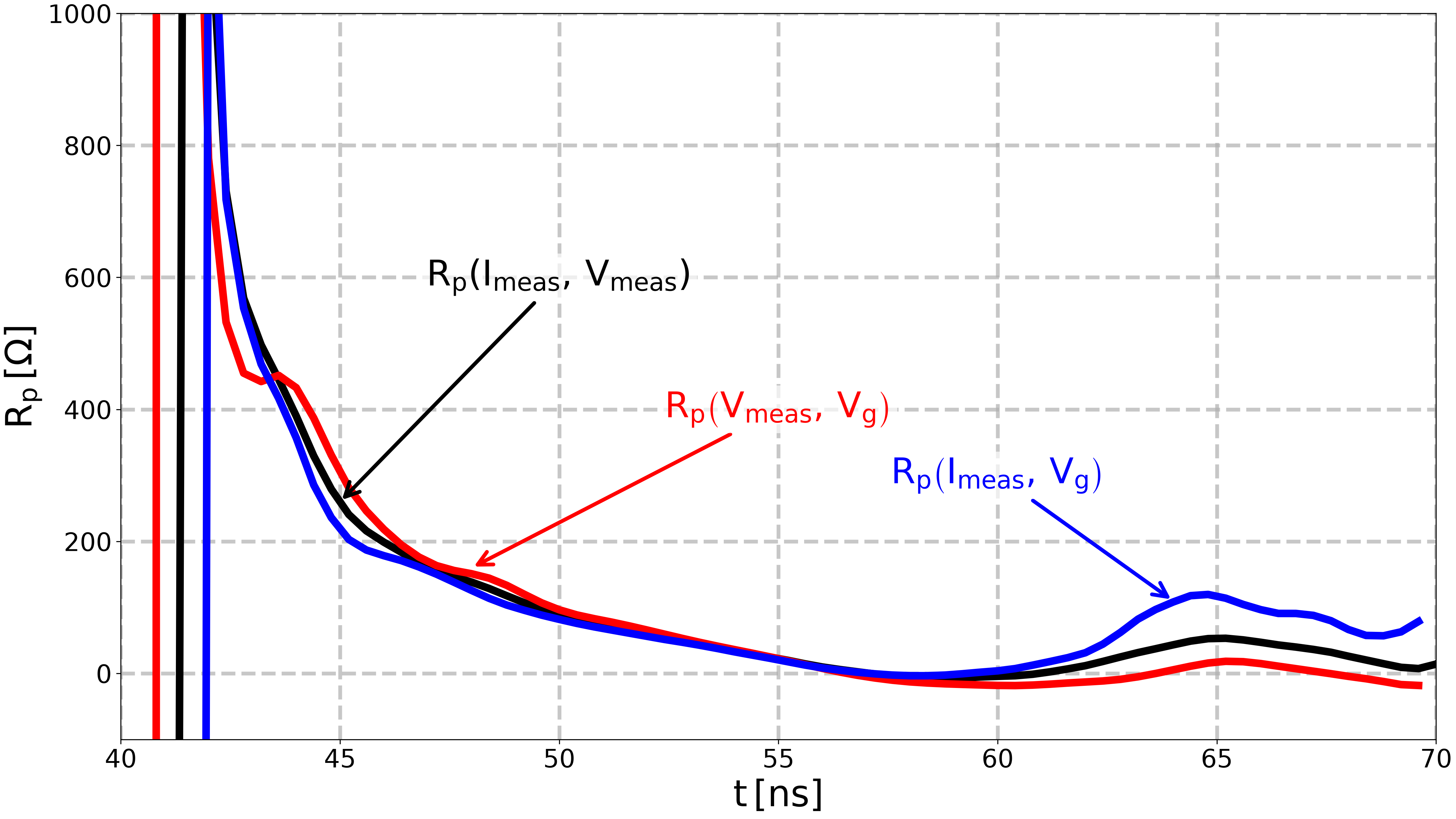
Comparison of formulas to extracte plasma resistance.

In this example, the plasma is assumed to be a time-varying resistance.

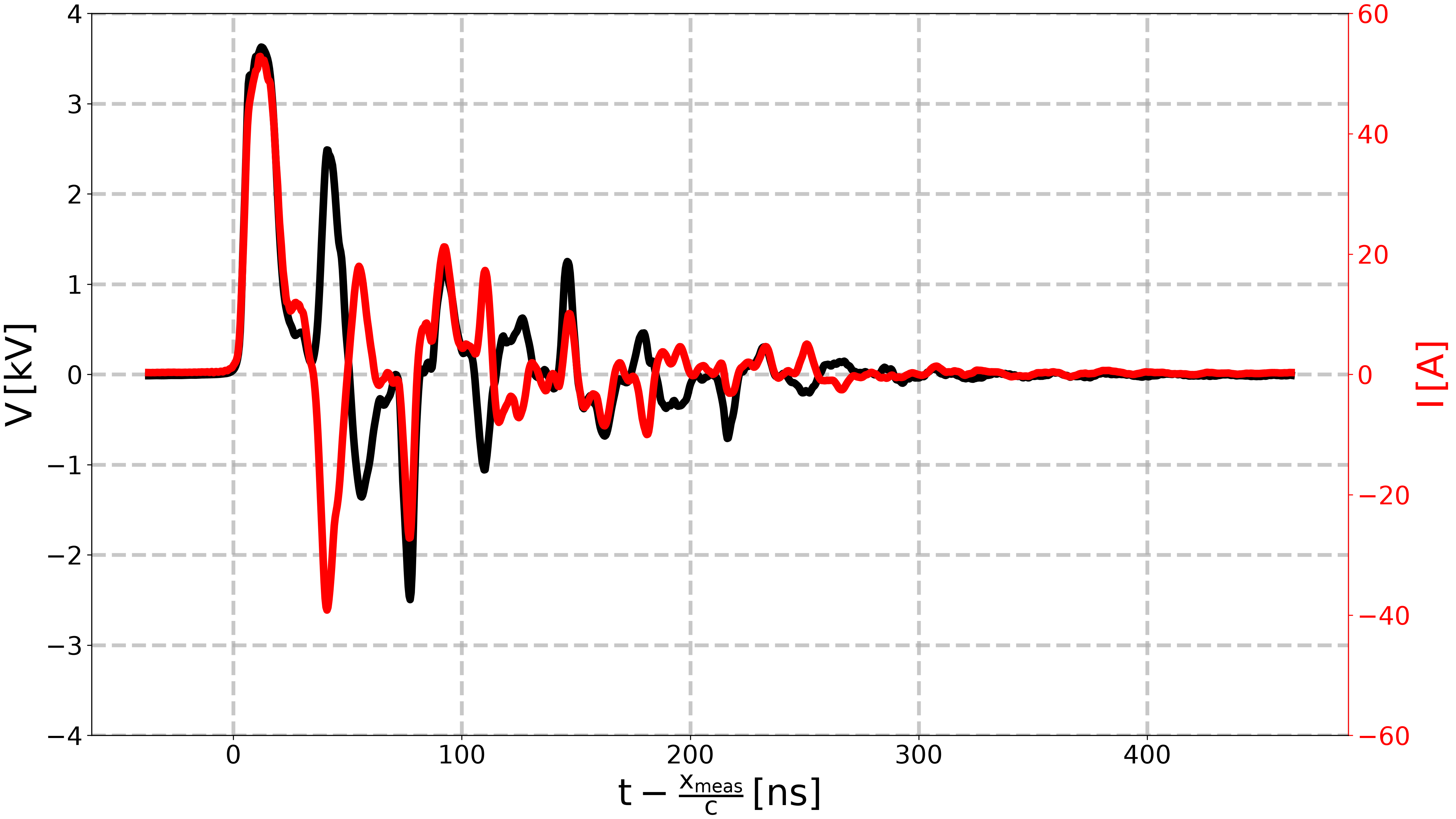
Experimental data of [Minesi2022] are used to extract the plasma resistance. For the remote configuration case, voltage and current signals are measured at the middle of a cable of length \(L \approx 6 \, \mathrm{m}\).

This example shows how to extract the resistance of a plasma load from either:

• measured voltage and measured current, at the same position,

• measured voltage and knowledge of the generator voltage,

• measured current and knowledge of the generator voltage.

# This sets the fourth figure as the thumbnail for the example gallery.
# sphinx_gallery_thumbnail_number = 4
# This displays each image separately in the example gallery.
# sphinx_gallery_multi_image = "single"

First, we import the required libraries.

We start by importing the modules we need:

• matplotlib for drawing graphs,

• numpy for array functions,

• pyresiflex for the generator, load and transmission line.

import matplotlib.pyplot as plt
import numpy as np

from pyresiflex.experiment.purely_resistive_experiment import (
    PurelyResistiveExperiment,
)
from pyresiflex.generator.generator_real_impedance import (
    FromMeasurementGenerator,
)
from pyresiflex.misc.load_data import load_minesi_data
from pyresiflex.misc.plot import plot_voltage_current, set_mpl_style
from pyresiflex.misc.utils import get_path_to_data

set_mpl_style(nb_columns=2)

Load [Minesi2022] experimental data of remote configuration.

# Load the raw data from Figure 16 of [Minesi2022]_.
file = get_path_to_data(
    "Minesi2022",
    "fig16_remoteConfiguration.csv",
)
data = np.loadtxt(file, skiprows=3, delimiter=";")
times_raw = data[:, 0] * 1e-9  # [s]
voltages_raw = data[:, 1] * 1e3  # [V]
currents_raw = data[:, 3]  # [A]


# Plot the raw data.
fig, ax_v, ax_i = plot_voltage_current(
    voltage_time=times_raw,
    voltage_value=voltages_raw,
    current_time=times_raw,
    current_value=currents_raw,
)
ax_v.set_xlabel(r"$\mathregular{t - \frac{x_{meas}}{c} \, [ns]}$")
ax_v.set_ylim(-4, 4)
ax_i.set_ylim(-60, 60)

plt.show()

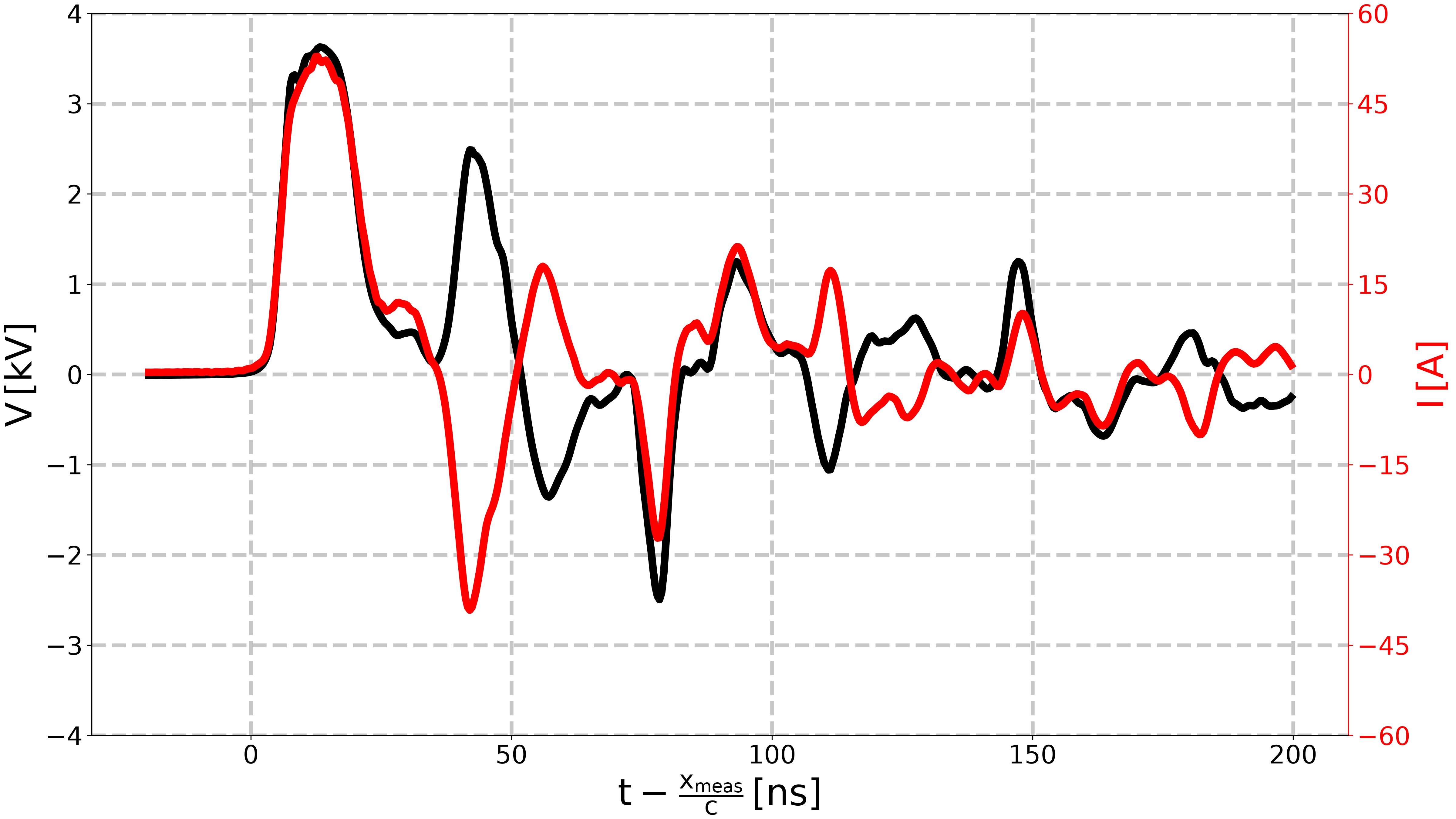
Preprocess the data.

# Define the zero at the first time the voltage reaches `threshold_voltage`.
threshold_voltage = 25  # [V]
idx_first = np.where(np.abs(voltages_raw) > threshold_voltage)[0][0]
times_raw = times_raw - times_raw[idx_first]

# Define a time window to analyze.
lower_time_window = -20e-9  # [s]
upper_time_window = 200e-9  # [s]

# Limit the time window to [lower_time_window, upper_time_window]
idx_min_wanted_time = np.where(times_raw > lower_time_window)[0][0]
idx_max_wanted_time = np.where(times_raw > upper_time_window)[0][0]

# Limit the time, voltages and currents to the wanted period.
times_expe = times_raw[idx_min_wanted_time:idx_max_wanted_time]
voltages_expe = voltages_raw[idx_min_wanted_time:idx_max_wanted_time]
currents_expe = currents_raw[idx_min_wanted_time:idx_max_wanted_time]

# Compute the energy from the voltage and current.
energies_expe = np.zeros_like(times_expe)  # [J]
for i in range(len(times_expe)):
    energies_expe[i] = np.trapezoid(
        voltages_expe[:i] * currents_expe[:i], times_expe[:i]
    )


# Plot the preprocessed data.
fig, ax_v, ax_i = plot_voltage_current(
    voltage_time=times_expe,
    voltage_value=voltages_expe,
    current_time=times_expe,
    current_value=currents_expe,
)
ax_v.set_xlabel(r"$\mathregular{t - \frac{x_{meas}}{c} \, [ns]}$")
ax_v.set_ylim(-4, 4)
ax_i.set_ylim(-60, 60)
ax_i.set_yticks([-60, -45, -30, -15, 0, 15, 30, 45, 60])

plt.show()

Transmission line parameters

# Transmission line parameters estimated from experimental data.
# See `plot_determine_Minesi2022_parameters.py` example for more details.
data = load_minesi_data()

# Length of the transmission line
L = data.L  # [m]
# Measurement points = probe positions
x = data.x_meas  # [m]
# Here, we assume that the probes are located at the same position.
x_meas_voltage = x_meas_current = x  # [m]
# Velocity of propagation of the wave in the cable.
c = data.c  # [m/s]
# Cable characteristic impedance.
Z_c = data.Z_c  # [Ohm]

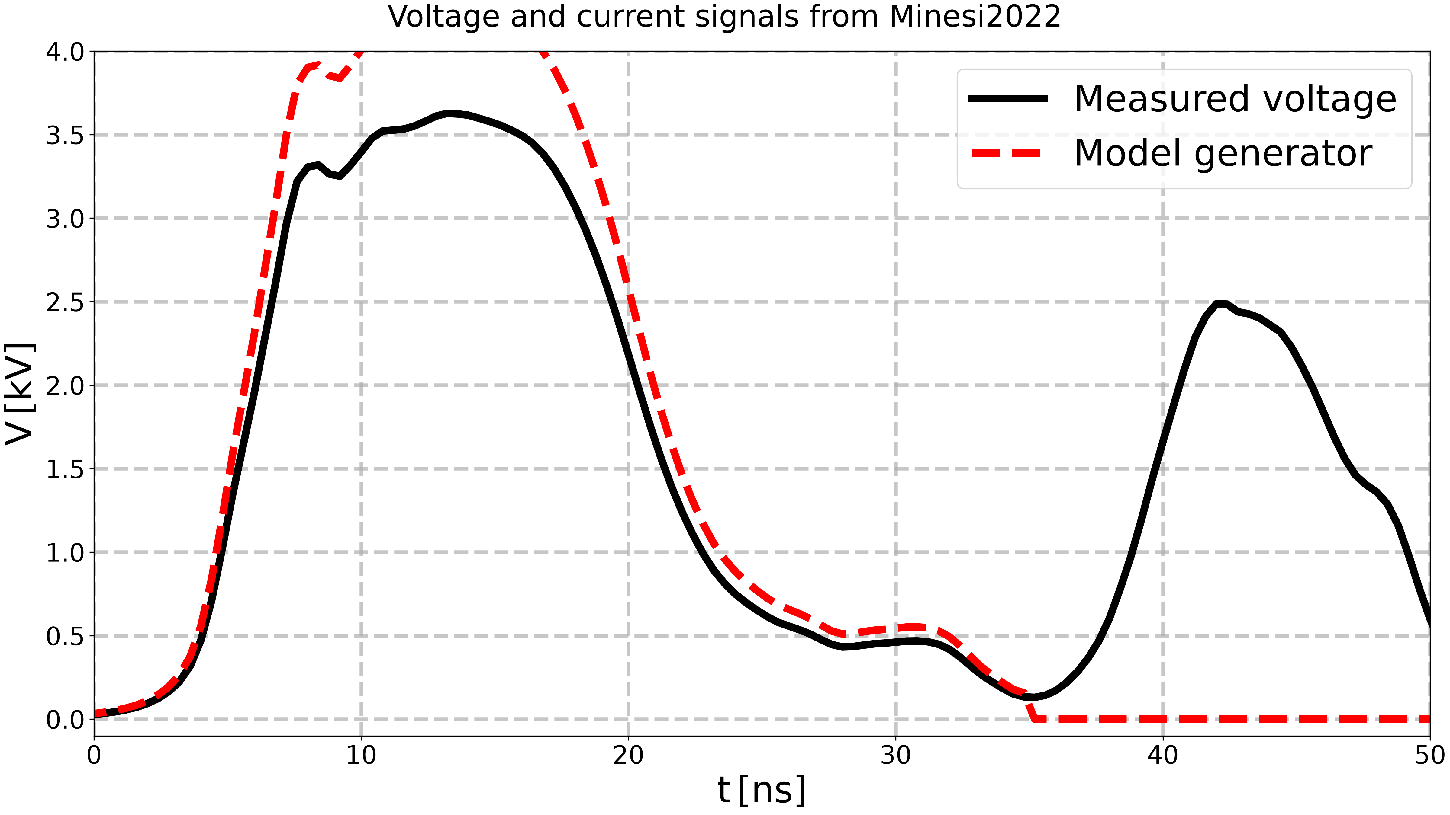
Generator parameters

# Impedance of the generator.
R_g = data.R_g  # [Ohm]
# Attenuation coefficient.
alpha_g = data.alpha_g  # [-]
# Pulse duration.
pulse_duration = 35e-9  # [s]


def V_meas_generator(t, times, voltages):
    if t < 0:
        return 0.0
    elif t > pulse_duration:
        return 0.0
    else:
        return np.interp(t, times, voltages) / alpha_g


generator = FromMeasurementGenerator(
    R_g=R_g, V_meas=lambda t: V_meas_generator(t, times_expe, voltages_expe)
)

# Plot the voltage signal.
fig, ax = plt.subplots()
fig.suptitle("Voltage and current signals from Minesi2022")
ax.plot(
    times_expe * 1e9,
    voltages_expe * 1e-3,
    color="black",
    label="Measured voltage",
)
ax.plot(
    times_expe * 1e9,
    [generator.generator_voltage(t) * 1e-3 for t in times_expe],
    "--",
    label="Model generator",
    color="red",
)
ax.set_xlabel(r"$\mathregular{t \, [ns]}$")
ax.set_ylabel(r"$\mathregular{V \, [kV]}$")
ax.set_xlim(0, 50)
ax.set_ylim(-0.1, 4.0)
ax.legend()
plt.show()

Compute the resistance from the voltage and current signals.

This is possible since the voltage and current signals are measured at the same position.

expe = PurelyResistiveExperiment(
    experimental_voltage_time=times_expe,
    experimental_voltage_value=voltages_expe,
    x_meas_voltage=x_meas_voltage,
    experimental_current_time=times_expe,
    experimental_current_value=currents_expe,
    x_meas_current=x_meas_current,
    L=L,
    Z_c=Z_c,
    c=c,
    correct_time_zero=True,
)

# Compute R_p(vmeas, imeas).
expe.compute_plasma_resistance_from_vmeas_and_imeas(
    times_expe, threshold=400, channel_formation_time=42e-9
)
# Compute R_p(vmeas, vg).
reconstructed_resistance_voltage = (
    expe.compute_plasma_resistance_from_vmeas_and_vg(
        times_expe,
        generator=generator,
    )
)
# Compute R_p(imeas, vg).
reconstructed_resistance_current = (
    expe.compute_plasma_resistance_from_imeas_and_vg(
        times_expe,
        generator=generator,
    )
)


# Plot R_p(vmeas, imeas).
fig, ax = expe.plot_resistance(
    times=times_expe,
    plot_whole=True,
    plot_corrected=False,
    plot_interpolated=False,
    show=False,
    legend=False,
)
# Change color of the first plot to black.
line = ax.get_lines()[0]
line.set_color("k")

# Plot R_p(vmeas, vg).
ax.plot(
    times_expe * 1e9,
    reconstructed_resistance_voltage,
    color="r",
    ls="-",
)
# Plot R_p(imeas, vg).
ax.plot(
    times_expe * 1e9,
    reconstructed_resistance_current,
    color="b",
    ls="-",
)
ax.set_xlim(40, 70)
ax.set_ylim(-100, 1000)

# Annotate the plot.
kwargs = dict(
    textcoords="data",
    fontsize=28,
    horizontalalignment="center",
    verticalalignment="center",
    bbox=dict(facecolor="white", alpha=0.7, edgecolor="none"),
)
ax.annotate(
    r"$\mathregular{R_p \left( I_{meas}, \, V_{meas} \right)}$",
    xytext=(50, 600),
    xy=(45, 260),
    color="k",
    arrowprops=dict(arrowstyle="->", color="k", lw=3),
    **kwargs,  # type: ignore
)
ax.annotate(
    r"$\mathregular{R_p \left( V_{meas}, \, V_g \right)}$",
    xytext=(55, 400),
    xy=(48, 160),
    color="r",
    arrowprops=dict(arrowstyle="->", color="r", lw=3),
    **kwargs,  # type: ignore
)
ax.annotate(
    r"$\mathregular{R_p \left( I_{meas}, \, V_g \right)}$",
    xytext=(60, 300),
    xy=(64, 110),
    color="b",
    arrowprops=dict(arrowstyle="->", color="b", lw=3),
    **kwargs,  # type: ignore
)

plt.show()

Save the figure.

# Export the image to a .svg file, in the figures folder.
fig.savefig(
    get_path_to_data(
        "article_figures",
        "Minesi2022_plasma_resistance_reconstruction_with_generator.svg",
        force_return=True,
    ),
)