Reproducing [Minesi2022] experiment.#
In this example, the plasma is a time-varying resistance.
Experimental data of [Minesi2022] are used to extract the plasma resistance. For the remote configuration case, voltage and current signals are measured at the middle of a cable of length \(L \approx 6 \, \mathrm{m}\).
To run the simulations, various parameters are needed:
for the transmission line:
Length \(L \approx 6 \, \mathrm{m}\)
Wave velocity \(c \approx 1.8 \times 10^8 \, \mathrm{m/s}\)
Characteristic impedance \(Z_c \approx 75 \, \Omega\)
for the generator:
Generator voltage equals to the first incident voltage multiplied by an attenuation factor \(\alpha_g\)
Internal resistance of \(R_g \approx 10 \, \Omega\)
for the load:
Plasma resistance is a time-varying resistance, whose values are automatically inferred from the measured voltage and current.
Then, the voltage and current at a given position of the cable are computed and compared to the experimental data.
# This sets the third figure as the thumbnail for the example gallery.
# sphinx_gallery_thumbnail_number = 5
# This displays each image separately in the example gallery.
# sphinx_gallery_multi_image = "single"
First, we import the required libraries.#
We start by importing the modules we need:
matplotlib for drawing graphs,
numpy for array functions,
pyresiflex for the generator, load and transmission line.
import matplotlib.pyplot as plt
import numpy as np
from adjustText import adjust_text

from pyresiflex.cable.cable import PerfectCable
from pyresiflex.experiment.purely_resistive_experiment import (
    PurelyResistiveExperiment,
)
from pyresiflex.generator.generator_real_impedance import (
    FromMeasurementGenerator,
)
from pyresiflex.misc.load_data import load_minesi_data
from pyresiflex.misc.plot import plot_voltage_current, set_mpl_style
from pyresiflex.misc.utils import get_path_to_data
from pyresiflex.solver.purely_resistive_solution import PurelyResistiveSolution

set_mpl_style(nb_columns=2)
Load [Minesi2022] experimental data of remote configuration.#
# Load the raw data from Figure 16 of [Minesi2022]_.
file = get_path_to_data(
    "Minesi2022",
    "fig16_remoteConfiguration.csv",
)
data = np.loadtxt(file, skiprows=3, delimiter=";")
times_raw = data[:, 0] * 1e-9  # [s]
voltages_raw = data[:, 1] * 1e3  # [V]
currents_raw = data[:, 3]  # [A]

# Plot the raw data.
fig, ax_v, ax_i = plot_voltage_current(
    voltage_time=times_raw,
    voltage_value=voltages_raw,
    current_time=times_raw,
    current_value=currents_raw,
)
ax_v.set_xlabel(r"$\mathregular{t - \frac{x_{meas}}{c} \, [ns]}$")
ax_v.set_ylim(-4, 4)
ax_i.set_ylim(-60, 60)

plt.show()
Preprocess the data.#
# Define the zero at the first time the voltage reaches `threshold_voltage`.
threshold_voltage = 25  # [V]
idx_first = np.where(np.abs(voltages_raw) > threshold_voltage)[0][0]
times_raw = times_raw - times_raw[idx_first]

# Define a time window to analyze.
lower_time_window = -20e-9  # [s]
upper_time_window = 200e-9  # [s]

# Limit the time window to [lower_time_window, upper_time_window]
idx_min_wanted_time = np.where(times_raw > lower_time_window)[0][0]
idx_max_wanted_time = np.where(times_raw > upper_time_window)[0][0]

# Limit the time, voltages and currents to the wanted period.
times_expe = times_raw[idx_min_wanted_time:idx_max_wanted_time]
voltages_expe = voltages_raw[idx_min_wanted_time:idx_max_wanted_time]
currents_expe = currents_raw[idx_min_wanted_time:idx_max_wanted_time]

# Compute the energy from the voltage and current.
energies_expe = np.zeros_like(times_expe)  # [J]
for i in range(len(times_expe)):
    energies_expe[i] = np.trapezoid(
        voltages_expe[:i] * currents_expe[:i], times_expe[:i]
    )


# Plot the preprocessed data.
fig, ax_v, ax_i = plot_voltage_current(
    voltage_time=times_expe,
    voltage_value=voltages_expe,
    current_time=times_expe,
    current_value=currents_expe,
)
ax_v.set_xlabel(r"$\mathregular{t - \frac{x_{meas}}{c} \, [ns]}$")
ax_v.set_xlim(0, 200)
ax_v.set_ylim(-4, 4)
ax_i.set_ylim(-60, 60)
ax_i.set_yticks([-60, -45, -30, -15, 0, 15, 30, 45, 60])

plt.show()

# Save the figure.
fig.savefig(
    get_path_to_data(
        "article_figures",
        "Minesi2022_voltage_current_experimental_measurement.svg",
        force_return=True,
    ),
)
Transmission line parameters.#
# Transmission line parameters estimated from experimental data.
# See `plot_determine_Minesi2022_parameters.py` example for more details.
data = load_minesi_data()

# Length of the transmission line
L = data.L  # [m]
# Measurement points = probe positions
x = data.x_meas  # [m]
# Here, we assume that the probes are located at the same position.
x_meas_voltage = x_meas_current = x  # [m]
# Velocity of propagation of the wave in the cable.
c = data.c  # [m/s]
# Cable characteristic impedance.
Z_c = data.Z_c  # [Ohm]

cable = PerfectCable(
    L=L,
    Z_c=Z_c,
    c=c,
)
Generator parameters.#
# Impedance of the generator.
R_g = data.R_g  # [Ohm]
# We can also test the sensitivity of the results to the value of R_g, by
# trying different values of R_g in a reasonable range.
R_g_low = 5  # [Ohm]
R_g_high = 20  # [Ohm]

# Attenuation coefficient.
alpha_g = data.alpha_g  # [-]
alpha_g_low = Z_c / (Z_c + R_g_low)  # [-]
alpha_g_high = Z_c / (Z_c + R_g_high)  # [-]


# Pulse duration.
pulse_duration = 35e-9  # [s]


def V_meas_generator(t, times, voltages, alpha):
    if t < 0:
        return 0.0
    elif t > pulse_duration:
        return 0.0
    else:
        return np.interp(t, times, voltages) / alpha


generator = FromMeasurementGenerator(
    R_g=R_g,
    V_meas=lambda t: V_meas_generator(t, times_expe, voltages_expe, alpha_g),
)
generator_low = FromMeasurementGenerator(
    R_g=R_g_low,
    V_meas=lambda t: V_meas_generator(
        t, times_expe, voltages_expe, alpha_g_low
    ),
)
generator_high = FromMeasurementGenerator(
    R_g=R_g_high,
    V_meas=lambda t: V_meas_generator(
        t, times_expe, voltages_expe, alpha_g_high
    ),
)

# Plot the voltage signal.
set_mpl_style(nb_columns=1)
fig, ax = plt.subplots()
ax.plot(
    times_expe * 1e9,
    voltages_expe * 1e-3,
    color="black",
    label="Measured voltage",
)
ax.plot(
    times_expe * 1e9,
    [generator.generator_voltage(t) * 1e-3 for t in times_expe],
    "--",
    label="Model generator",
    color="red",
)
ax.set_xlabel(r"$\mathregular{t \, [ns]}$")
ax.set_ylabel(r"$\mathregular{V \, [kV]}$")
ax.set_xlim(0, 50)
ax.set_ylim(-0.1, 4.5)
ax.legend()
plt.show()

# Save the figure.
fig.savefig(
    get_path_to_data(
        "article_figures",
        "Minesi2022_generator_voltage_model.svg",
        force_return=True,
    ),
)
Load parameters.#
expe = PurelyResistiveExperiment(
    experimental_voltage_time=times_expe,
    experimental_voltage_value=voltages_expe,
    x_meas_voltage=x_meas_voltage,
    experimental_current_time=times_expe,
    experimental_current_value=currents_expe,
    x_meas_current=x_meas_current,
    L=L,
    Z_c=Z_c,
    c=c,
    correct_time_zero=True,
)

threshold_voltage_for_resistance = 0.2 * np.max(voltages_expe)  # [V]
expe.compute_plasma_resistance_from_vmeas_and_imeas(
    times_expe,
    threshold=threshold_voltage_for_resistance,
    channel_formation_time=42e-9,
    interpolate_with_previous_value=False,
)

plasma_load = expe.load_corrected

# Plot the plasma resistance.
set_mpl_style(nb_columns=1)
fig, ax = expe.plot_resistance(times=times_expe, plot_whole=True)
ax.set_xlim(40, 200)
ax.set_ylim(-100, 1000)
plt.show()

# Save the figure.
fig.savefig(
    get_path_to_data(
        "article_figures",
        "Minesi2022_plasma_resistance_with_time.svg",
        force_return=True,
    ),
)
Solution object.#
solution = PurelyResistiveSolution(
    generator=generator,
    load=plasma_load,
    cable=cable,
)

solution_low = PurelyResistiveSolution(
    generator=generator_low,
    load=plasma_load,
    cable=cable,
)
solution_high = PurelyResistiveSolution(
    generator=generator_high,
    load=plasma_load,
    cable=cable,
)

# ########################################################################
# ########################################################################
# ###################  REMOTE CONFIGURATION ##############################
# ########################################################################
# ########################################################################
Compute voltage, current and energy at remote configuration.#
# Time vector for the simulation.
nb_steps = 1000
times = np.linspace(lower_time_window, upper_time_window, nb_steps)  # [s]

# Compute the voltage and current at probes' position.
solution.solve(x, times)

voltages = solution.voltage  # [V]
currents = solution.current  # [A]
energies = solution.energy  # [J]
xs = solution.x  # [m]
times = solution.t  # [s]
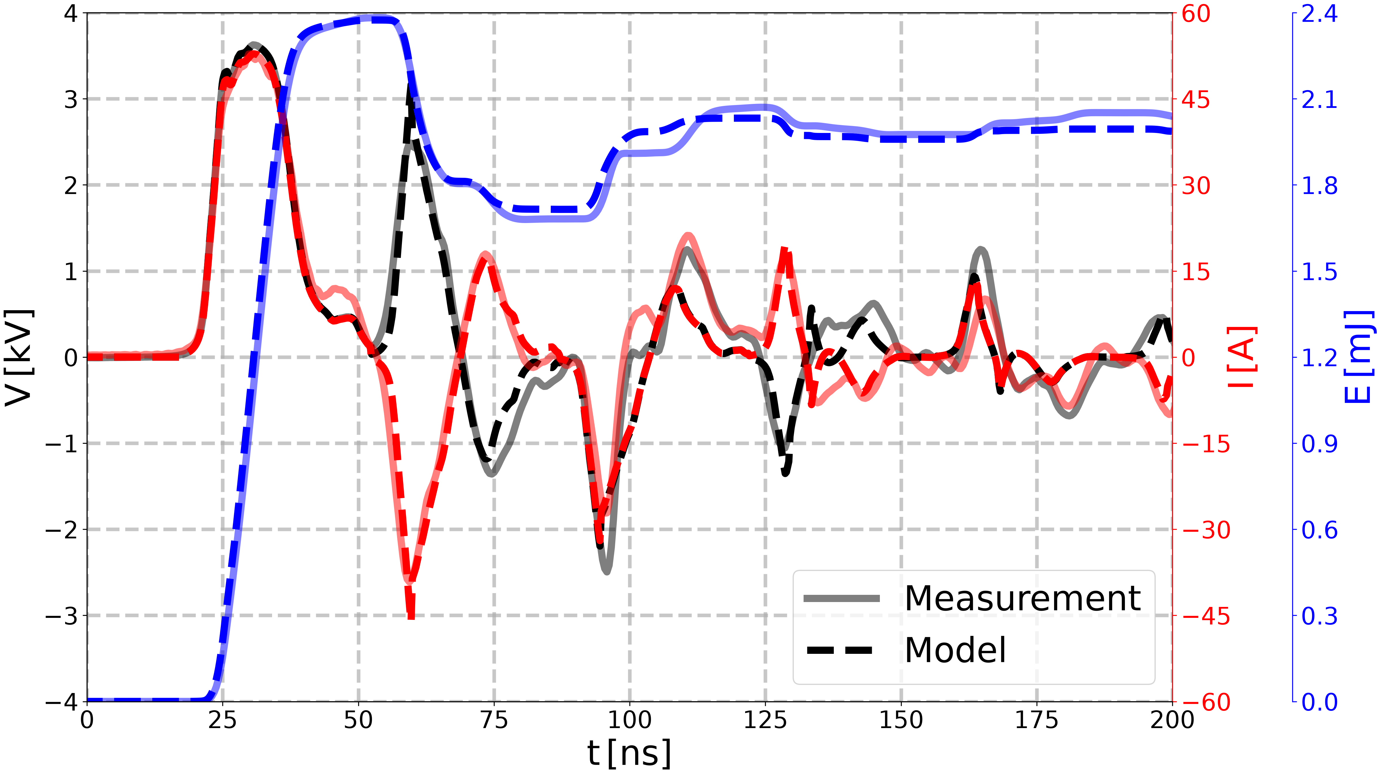
Plot voltage, current, and energy at remote configuration.#
# Do we want to plot the current and energy?
plot_current = True
plot_energy = True
# Do we want to shift the time axis to have t - x/c?
shift_time_axis = False

if shift_time_axis:
    times_shifted = times - x / c
    times_expe_shifted = times_expe
    x_label = r"$\mathregular{t - \frac{x_{meas}}{c} \, [ns]}$"
else:
    times_shifted = times
    times_expe_shifted = times_expe + x / c
    x_label = r"$\mathregular{t \, [ns]}$"

set_mpl_style(nb_columns=2)
fig, ax_v = plt.subplots()

# Plot voltage.
plot_line_v = ax_v.plot(
    times_shifted * 1e9,
    voltages * 1e-3,
    color="k",
    ls="--",
    label="Voltage (computed)",
)
plot_line_v_measured = ax_v.plot(
    times_expe_shifted * 1e9,
    voltages_expe * 1e-3,
    color="k",
    label="Voltage (experimental)",
    alpha=0.5,
)
# .. Plot options for voltage.
ax_v.set_xlabel(x_label)
ax_v.set_ylabel(r"$\mathregular{V \, [kV]}$")
ax_v.set_ylim(-4, 4)
ax_v.spines["left"].set_color("k")
ax_v.set_xlim(0, times_shifted[-1] * 1e9)

# Plot current.
if plot_current:
    ax_i = ax_v.twinx()
    ax_i.plot(
        times_shifted * 1e9,
        currents,
        color="r",
        ls="--",
        label="Current (computed)",
    )
    ax_i.plot(
        times_expe_shifted * 1e9,
        currents_expe,
        color="r",
        label="Current (experimental)",
        alpha=0.5,
    )
    # .. Plot options for current.
    ax_i.set_ylabel(r"$\mathregular{I \, [A]}$", color="r")
    # ax_i.set_ylim(-max_abs_current, max_abs_current)
    ax_i.set_ylim(-60, 60)
    ax_i.grid(visible=False)
    # Change color of the right y-axis to red.
    ax_i.spines["right"].set_color("r")
    # Also change the color of the ticks.
    ax_i.tick_params(axis="y", colors="r")
    # Move x-position of the y-label.
    ax_i.yaxis.set_label_coords(1.05, 0.5)
    # Set y-ticks for current.
    ax_i.set_yticks([-60, -45, -30, -15, 0, 15, 30, 45, 60])

# Plot energy.
if plot_energy:
    ax_e = ax_v.twinx()
    ax_e.plot(
        times_shifted * 1e9,
        energies * 1e3,
        color="b",
        ls="--",
        label="Energy",
    )
    ax_e.plot(
        times_expe_shifted * 1e9,
        energies_expe * 1e3,
        color="b",
        label="Energy (experimental)",
        alpha=0.5,
    )
    # .. Plot options for energy.
    ax_e.set_ylabel(r"$\mathregular{E \, [mJ]}$", color="b")
    # Move the y-axis of ax_e to the right, by 100 points
    ax_e.spines["right"].set_position(("outward", 100))
    ax_e.grid(visible=False)
    ax_e.set_ylim(0, 2.4)
    ax_e.set_yticks([0, 0.3, 0.6, 0.9, 1.2, 1.5, 1.8, 2.1, 2.4])
    # Change color of the right y-axis to blue.
    ax_e.spines["right"].set_color("b")
    # Also change the color of the ticks.
    ax_e.tick_params(axis="y", colors="b")


ax_v.legend(
    handles=plot_line_v_measured + plot_line_v,
    labels=["Measurement", "Model"],
    loc="lower right",
)

plt.show()

# Save the figure.
fig.savefig(
    get_path_to_data(
        "article_figures",
        f"Minesi2022_comparison_remote_configuration__Rg_{R_g}_Ohm.svg",
        force_return=True,
    ),
)
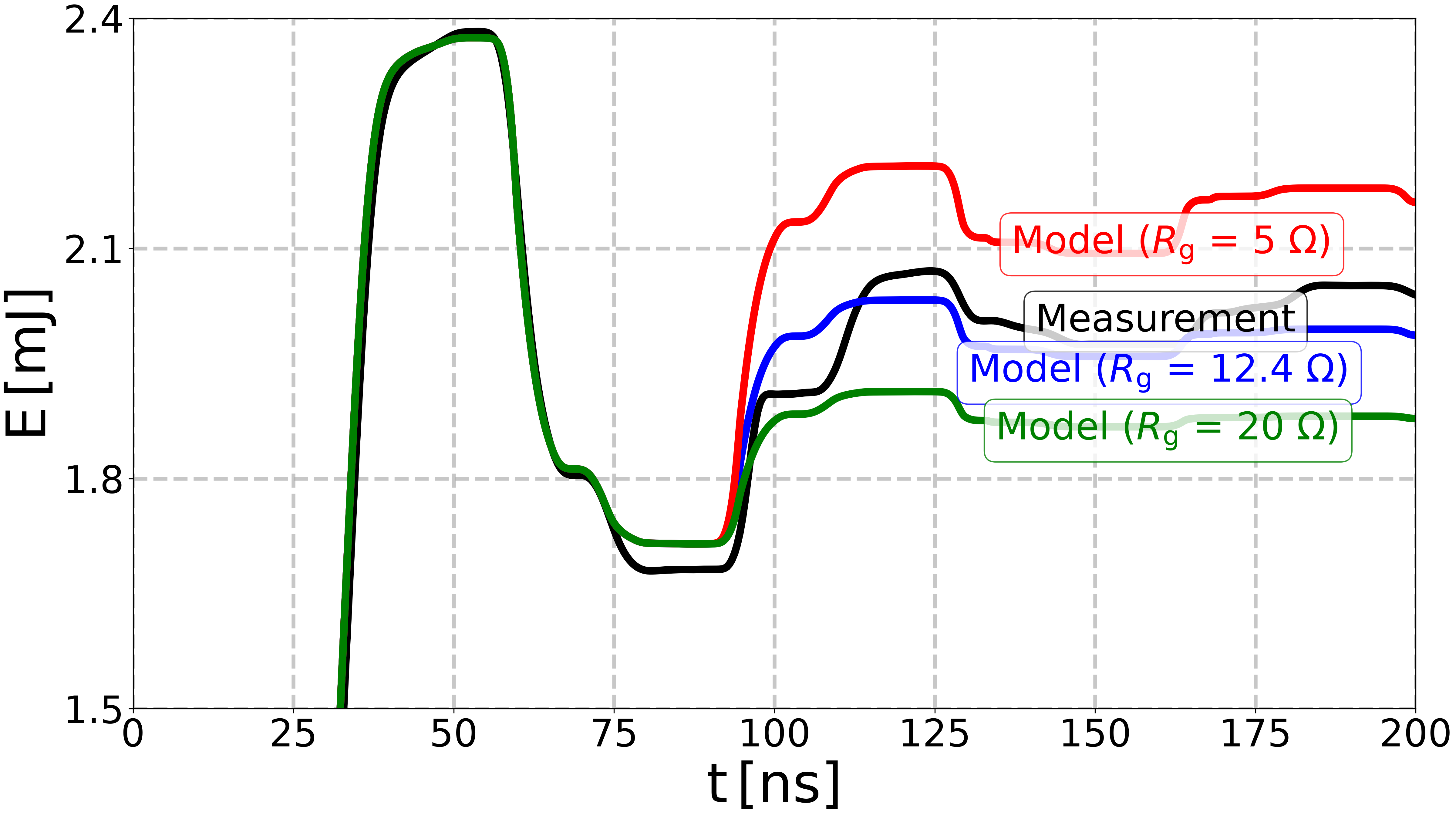
Compute and plot voltage, current and energy (sensitivity analysis).#
# Time vector for the simulation.
nb_steps = 1000
times = np.linspace(lower_time_window, upper_time_window, nb_steps)  # [s]

# Compute the voltage and current at probes' position.
solution_low.solve(x, times)
solution_high.solve(x, times)

# Do we want to shift the time axis to have t - x/c?
shift_time_axis = False

if shift_time_axis:
    times_shifted = times - x / c
    times_expe_shifted = times_expe
    x_label = r"$\mathregular{t - \frac{x_{meas}}{c} \, [ns]}$"
else:
    times_shifted = times
    times_expe_shifted = times_expe + x / c
    x_label = r"$\mathregular{t \, [ns]}$"

set_mpl_style(nb_columns=1)
fig, ax_e = plt.subplots()

# Plot energy, with a label for each curve at a specific time (e.g., 175 ns).
texts = []
for time, energy, color, label in zip(
    [times_expe_shifted, times_shifted, times_shifted, times_shifted],
    [energies_expe, energies, solution_low.energy, solution_high.energy],
    ["k", "b", "r", "g"],
    [
        "Measurement",
        r"Model ($R_\text{g}$" + f" = {R_g:.1f} Ω)",
        r"Model ($R_\text{g}$" + f" = {R_g_low} Ω)",
        r"Model ($R_\text{g}$" + f" = {R_g_high} Ω)",
    ],
):
    wanted_time = 160e-9  # [s]
    idx_wanted = np.where(time > wanted_time)[0][0]

    ax_e.plot(
        time * 1e9,
        energy * 1e3,
        color=color,
    )
    texts.append(
        ax_e.text(
            wanted_time * 1e9,
            float(energy[idx_wanted] * 1e3),
            label,
            color=color,
            ha="center",
            va="center",
            bbox=dict(
                facecolor="white",
                alpha=0.8,
                edgecolor=color,
                boxstyle="round",
            ),
        )
    )


# Plot options for energy.
ax_e.set_xlim(0, 200)
ax_e.set_xlabel(x_label)

ax_e.set_yticks([1.5, 1.8, 2.1, 2.4])
ax_e.set_ylim(1.5, 2.4)
ax_e.set_ylabel(r"$\mathregular{E \, [mJ]}$")
adjust_text(texts, avoid_self=False)

plt.show()

# Save the figure.
fig.savefig(
    get_path_to_data(
        "article_figures",
        "Minesi2022_comparison_remote_configuration_sensitivity.svg",
        force_return=True,
    ),
)

# ########################################################################
# ########################################################################
# ####################  ANODE CONFIGURATION ##############################
# ########################################################################
# ########################################################################
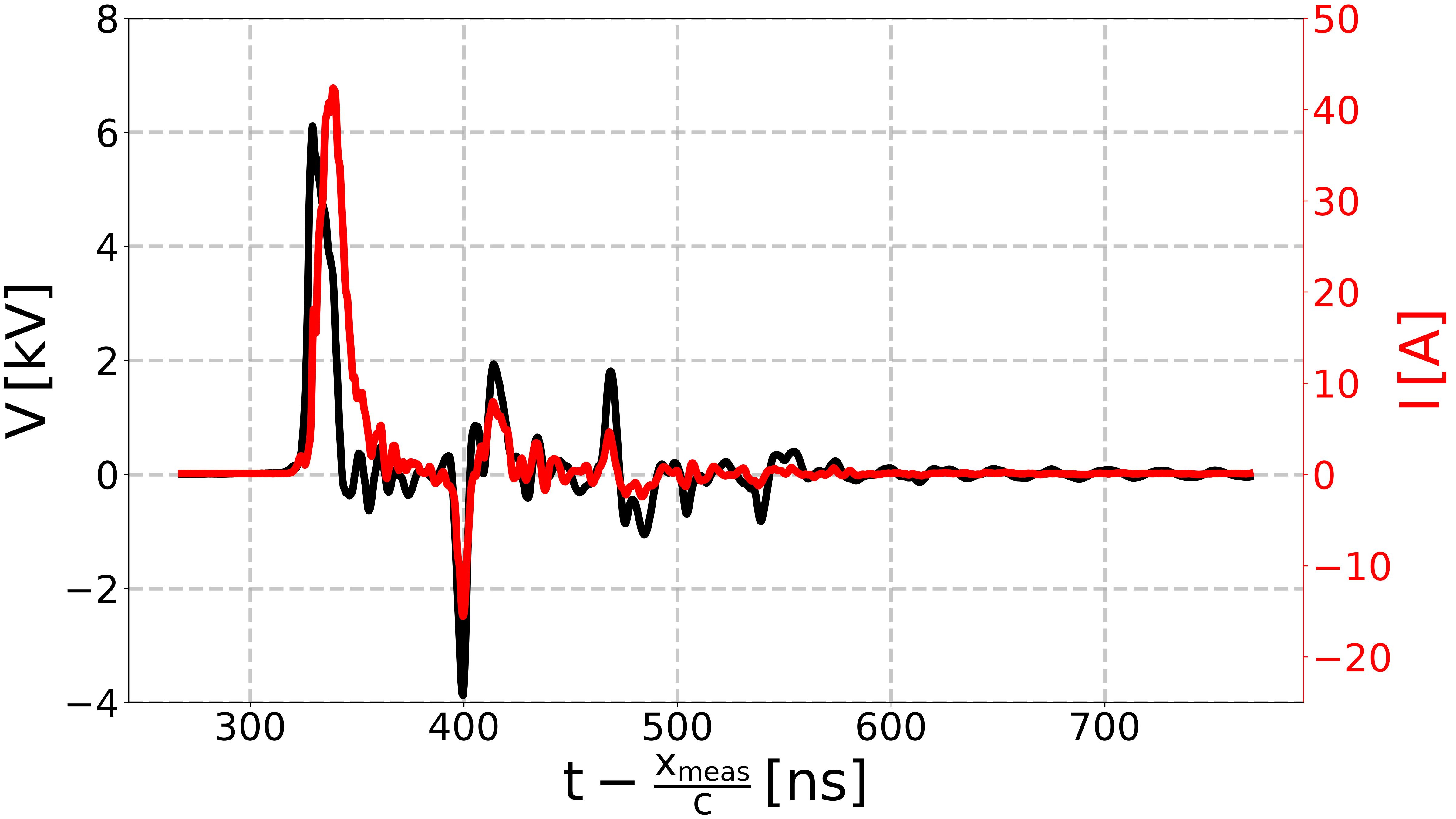
Load [Minesi2022] experimental data of anode configuration.#
# Load the raw data from Figure 16 of [Minesi2022]_.
file = get_path_to_data(
"Minesi2022",
"fig3_anodeConfiguration.csv",
)
data = np.loadtxt(file, skiprows=3, delimiter=";")
times_raw_anode = data[:, 0] # [s]
voltages_raw_anode = data[:, 1] * 1e3 # [V]
currents_raw_anode = data[:, 2] # [A]
# Plot the raw data.
fig, ax_v, ax_i = plot_voltage_current(
voltage_time=times_raw_anode,
voltage_value=voltages_raw_anode,
current_time=times_raw_anode,
current_value=currents_raw_anode,
)
ax_v.set_xlabel(r"$\mathregular{t - \frac{x_{meas}}{c} \, [ns]}$")
ax_v.set_ylim(-4, 8)
ax_i.set_ylim(-25, 50)
plt.show()
# Define the zero at the first time the voltage reaches `threshold_voltage`.
threshold_voltage = 140 # [V]
idx_first = np.where(np.abs(voltages_raw_anode) > threshold_voltage)[0][0]
times_raw_anode = times_raw_anode - times_raw_anode[idx_first]
# Define a time window to analyze.
lower_time_window = -20e-9 # [s]
upper_time_window = 200e-9 # [s]
# Limit the time window to [lower_time_window, upper_time_window]
idx_min_wanted_time = np.where(times_raw_anode > lower_time_window)[0][0]
idx_max_wanted_time = np.where(times_raw_anode > upper_time_window)[0][0]
# Limit the time, voltages and currents to the wanted period.
times_expe_anode = times_raw_anode[idx_min_wanted_time:idx_max_wanted_time]
voltages_expe_anode = voltages_raw_anode[
idx_min_wanted_time:idx_max_wanted_time
]
currents_expe_anode = currents_raw_anode[
idx_min_wanted_time:idx_max_wanted_time
]
# Compute the energy from the voltage and current.
energies_expe_anode = np.zeros_like(times_expe_anode) # [J]
for i in range(len(times_expe_anode)):
energies_expe_anode[i] = np.trapezoid(
voltages_expe_anode[:i] * currents_expe_anode[:i], times_expe_anode[:i]
)
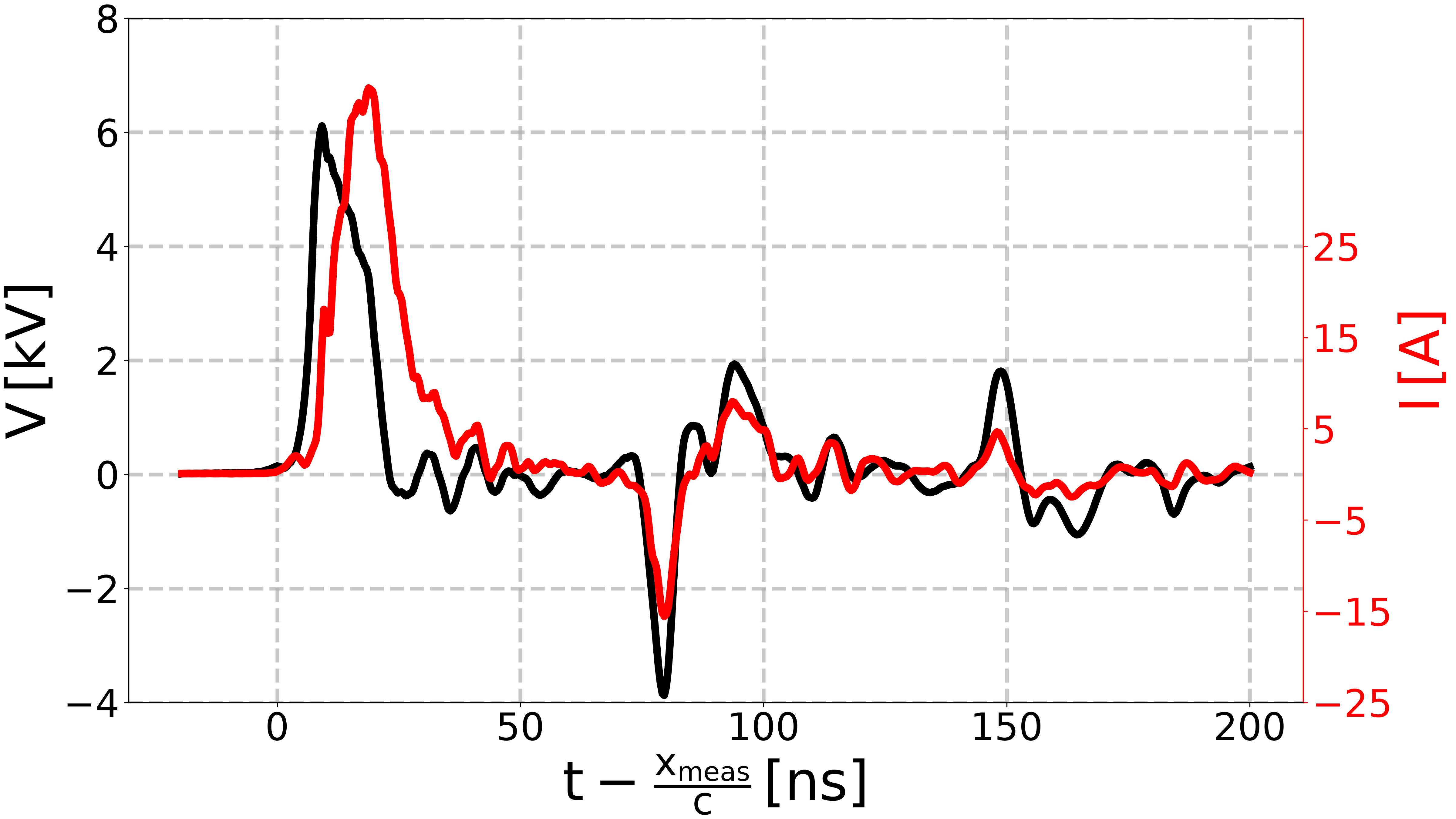
# Plot the preprocessed data.
fig, ax_v, ax_i = plot_voltage_current(
voltage_time=times_expe_anode,
voltage_value=voltages_expe_anode,
current_time=times_expe_anode,
current_value=currents_expe_anode,
)
ax_v.set_xlabel(r"$\mathregular{t - \frac{x_{meas}}{c} \, [ns]}$")
ax_v.set_ylim(-4, 8)
ax_i.set_ylim(-25, 50)
ax_i.set_yticks([-25, -15, -5, 5, 15, 25])
plt.show()
Compute voltage, current and energy at anode configuration.#
# Time vector for the simulation.
nb_steps = 1000
times = np.linspace(0, 200e-9, nb_steps)  # [s]
# Position of probes for measurement
x = 6.1  # [m]


# Compute the voltage and current at probes' position.
solution.solve(x, times)

voltages = solution.voltage  # [V]
currents = solution.current  # [A]
energies = solution.energy  # [J]
xs = solution.x  # [m]
times = solution.t  # [s]
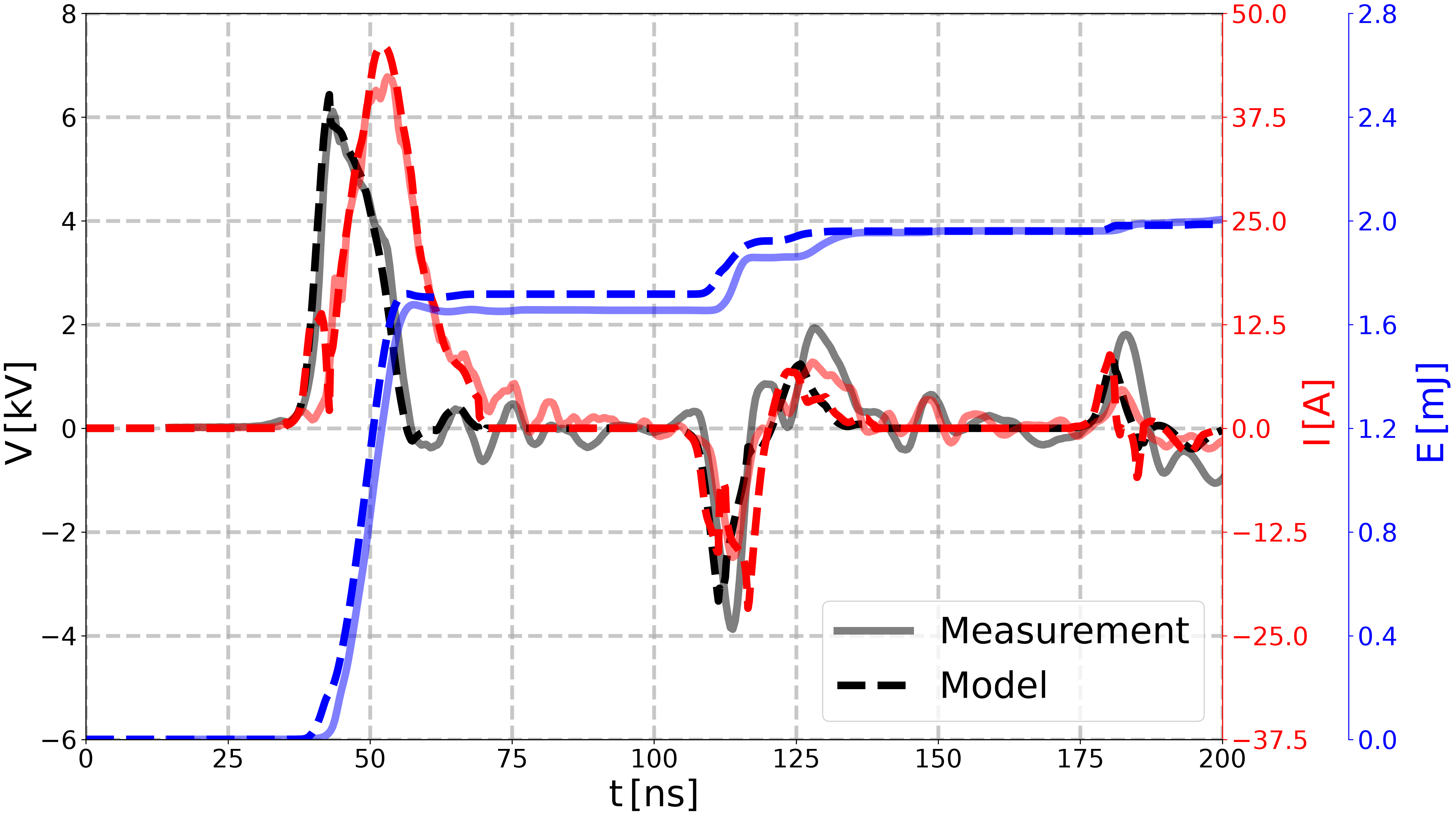
Plot voltage, current, and energy at anode configuration.#
set_mpl_style(nb_columns=2)
# Do we want to plot the current and energy?
plot_current = True
plot_energy = True
# Do we want to shift the time axis to have t - x/c?
shift_time_axis = False

if shift_time_axis:
    times_shifted = times - x / c
    times_expe_anode_shifted = times_expe_anode
    x_label = r"$\mathregular{t - \frac{x_{meas}}{c} \, [ns]}$"
else:
    times_shifted = times
    times_expe_anode_shifted = times_expe_anode + x / c
    x_label = r"$\mathregular{t \, [ns]}$"

fig, ax_v = plt.subplots()

# Plot voltage.
plot_line_v = ax_v.plot(
    times_shifted * 1e9,
    voltages * 1e-3,
    color="k",
    ls="--",
    label="Voltage (computed)",
)
plot_line_v_measured = ax_v.plot(
    times_expe_anode_shifted * 1e9,
    voltages_expe_anode * 1e-3,
    color="k",
    label="Voltage (experimental)",
    alpha=0.5,
)
# .. Plot options for voltage.
ax_v.set_xlabel(x_label)
ax_v.set_ylabel(r"$\mathregular{V \, [kV]}$")
ax_v.set_ylim(-6, 8)
ax_v.spines["left"].set_color("k")
ax_v.set_xlim(times_shifted[0] * 1e9, times_shifted[-1] * 1e9)
# Move position of the y-label.
ax_v.yaxis.set_label_coords(-0.04, 0.45)

# Plot current.
if plot_current:
    ax_i = ax_v.twinx()
    ax_i.plot(
        times_shifted * 1e9,
        currents,
        color="r",
        ls="--",
        label="Current (computed)",
    )
    ax_i.plot(
        times_expe_anode_shifted * 1e9,
        currents_expe_anode,
        color="r",
        label="Current (experimental)",
        alpha=0.5,
    )
    # .. Plot options for current.
    ax_i.set_ylabel(r"$\mathregular{I \, [A]}$", color="r")
    # ax_i.set_ylim(-max_abs_current, max_abs_current)
    ax_i.set_ylim(-37.5, 50)
    ax_i.set_yticks([-37.5, -25, -12.5, 0, 12.5, 25, 37.5, 50])
    ax_i.grid(visible=False)
    # Change color of the right y-axis to red.
    ax_i.spines["right"].set_color("r")
    # Also change the color of the ticks.
    ax_i.tick_params(axis="y", colors="r")
    # Move position of the y-label.
    ax_i.yaxis.set_label_coords(1.07, 0.45)

# Plot energy.
if plot_energy:
    ax_e = ax_v.twinx()
    ax_e.plot(
        times_shifted * 1e9,
        energies * 1e3,
        color="b",
        ls="--",
        label="Energy",
    )
    ax_e.plot(
        times_expe_anode_shifted * 1e9,
        energies_expe_anode * 1e3,
        color="b",
        label="Energy (experimental)",
        alpha=0.5,
    )
    # .. Plot options for energy.
    ax_e.set_ylabel(r"$\mathregular{E \, [mJ]}$", color="b")
    # Move the y-axis of ax_e to the right, by 100 points
    ax_e.spines["right"].set_position(("outward", 100))
    ax_e.grid(visible=False)
    ax_e.set_ylim(0, 2.8)
    ax_e.set_yticks([0, 0.4, 0.8, 1.2, 1.6, 2.0, 2.4, 2.8])
    # Change color of the right y-axis to blue.
    ax_e.spines["right"].set_color("b")
    # Also change the color of the ticks.
    ax_e.tick_params(axis="y", colors="b")
    # Move position of the y-label.
    ax_e.yaxis.set_label_coords(1.17, 0.45)


ax_v.legend(
    handles=plot_line_v_measured + plot_line_v,
    labels=["Measurement", "Model"],
    loc="lower right",
)

plt.show()

# Save the figure.
fig.savefig(
    get_path_to_data(
        "article_figures",
        f"Minesi2022_comparison_anode_configuration__Rg_{R_g}_Ohm.svg",
        force_return=True,
    ),
)


# # %%
# # Compute at different times for all positions and animate.
# # ---------------------------------------------------------

# # Define the space and time vectors.
# N_x = 100  # number of points in space.
# xs = np.linspace(0, L, N_x, dtype=float)  # Space vector [m]

# t_max = 200e-9  # Maximum time [s]
# N_t = 100  # Number of points in time.
# times = np.linspace(0, t_max, N_t, dtype=float)  # Time vector [s]

# solution.solve(xs, times)

# # Animate the voltage and current along the transmission line.
# ani = solution.animation()

# # Save the animation as a .mp4 file.
# ani.save("reproduce_Minesi2022_experiments.mp4", writer="ffmpeg", fps=20)

# # %%
# # Save the animation as a .gif file.
# import matplotlib.animation as animation  # noqa: E402

# writer = animation.PillowWriter(fps=15, bitrate=1800)
# ani.save("reproduce_Minesi2022_experiments.gif", writer=writer)
Total running time of the script: (0 minutes 7.814 seconds)