Cable length influence on electrical signals.

In experiments involving short pulse durations, like in Nanosecond Repetitive Pulsed (NRP) discharges, the influence of cable length on electrical signals is significant.

For long cable, a clear separation between incident and reflected signals can be observed. As the cable becomes shorter, superposition of signals will appear. At very short cable lengths, the incident and reflected signals will be indistinguishable, and the circuit will behave as if the generator is directly connected to the load (i.e., no transmission line effects).

This example setups a simulation to visualize these effects, with the following assumptions:

• Perfect transmission line behavior,

• Constant resistance load,

• Trapezoidal pulse shape.

# This sets the following figure as the thumbnail for the example gallery.
# sphinx_gallery_thumbnail_number = 3

First, we import the required libraries.

We start by importing the modules we need:

• matplotlib for drawing graphs,

• numpy for array functions,

• pyresiflex for the generator, load and transmission line.

import matplotlib.pyplot as plt
import numpy as np

from pyresiflex.cable.cable import PerfectCable
from pyresiflex.generator.generator_real_impedance import TrapezoidalGenerator
from pyresiflex.load.time_varying_resistance import ConstantResistance
from pyresiflex.misc.plot import save_figure, set_mpl_style
from pyresiflex.solver.purely_resistive_solution import PurelyResistiveSolution

set_mpl_style(nb_columns=1)

Generator parameters

trapezoidal_generator = TrapezoidalGenerator(
    R_g=0,  # Impedance of the generator [Ohm]
    U_off=0.0,  # Off voltage [V]
    U_on=10e3,  # On voltage [V]
    t_rise=3e-9,  # Rise time [s]
    t_on=10e-9,  # Time on [s]
    t_fall=3e-9,  # Fall time [s]
)

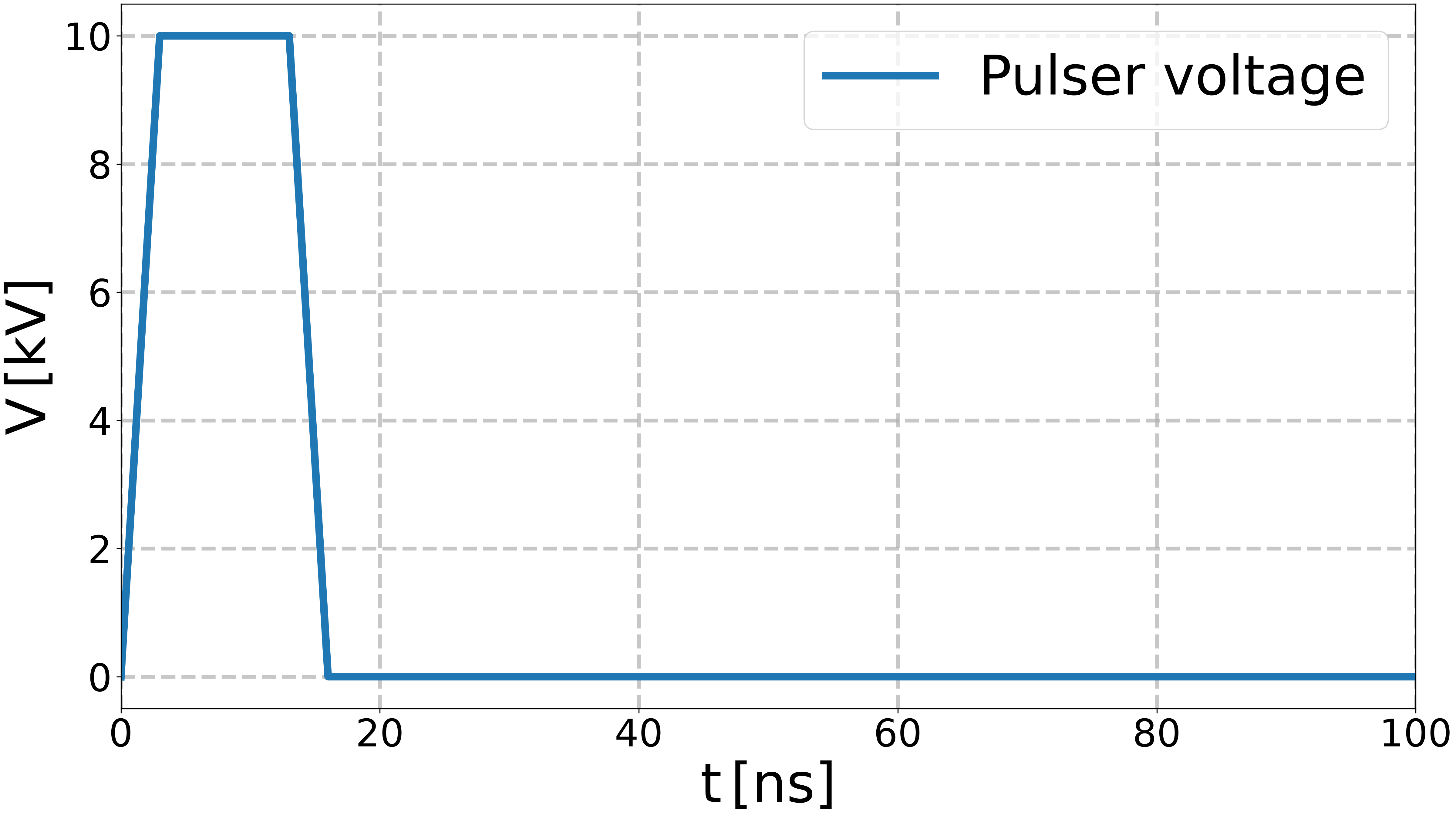
# Plot the generator voltage
# --------------------------

# Define time
times = np.arange(0, 100, 0.1) * 1e-9

generator_voltage = np.array(
    [trapezoidal_generator.generator_voltage(t) for t in times]
)

fig, ax = plt.subplots()
ax.plot(
    times * 1e9,
    generator_voltage * 1e-3,
    label="Pulser voltage",
)

ax.set_xlim(0, 100)
ax.set_xlabel(r"$\mathregular{t \, [ns]}$")
ax.set_ylabel(r"$\mathregular{V \, [kV]}$")
ax.legend()
ax.grid(visible=True)
plt.show()

Load parameters

Z = 50  # Constant resistance [Ohm]
plasma_load = ConstantResistance(Z)

Transmission line parameters

# Length of the transmission line.
cable_lengths = [0.1, 0.3, 0.5, 1, 2, 3, 4, 5, 6]  # [m]

c = 2e8  # Wave velocity [m/s]
Z_c = 75  # Characteristic impedance [Ohm]


cables: list[PerfectCable] = []
for L in cable_lengths:
    cable = PerfectCable(
        L=L,
        Z_c=Z_c,
        c=c,
    )
    cables.append(cable)

Solution object.

solutions: list[PurelyResistiveSolution] = []
for cable in cables:
    solution = PurelyResistiveSolution(
        generator=trapezoidal_generator,
        load=plasma_load,
        cable=cable,
    )
    solutions.append(solution)

# Compute voltage and current at a given position.
# ------------------------------------------------


# Solve the problem.
for solution in solutions:
    # Get the cable length.
    L = solution.cable.L

    # Position where measurements are taken [m].
    x_meas = L / 2  # Mid-point of the cable.

    # Time array for the simulation.
    start_time = 0  # Start time for the simulation [s].
    max_time = 10 * L / c  # Max time for the simulation [s].
    max_time = max(max_time, 50e-9)  # Ensure at least 50 ns for short cables.
    nb_points = 1_000  # Number of time points for the simulation.
    times = np.linspace(start_time, max_time, nb_points)  # Time array [s].

    print(f"Solving for cable length L = {L:.2f} m.")
    print(f"Measurement position x_meas = {x_meas:.2f} m.")
    print(
        f"Time array from {start_time:.2e} s to {max_time:.2e} s"
        f" with {nb_points} points."
    )
    print("---" * 20)

    solution.solve(x_meas, times)

Solving for cable length L = 0.10 m.
Measurement position x_meas = 0.05 m.
Time array from 0.00e+00 s to 5.00e-08 s with 1000 points.
------------------------------------------------------------
Solving for cable length L = 0.30 m.
Measurement position x_meas = 0.15 m.
Time array from 0.00e+00 s to 5.00e-08 s with 1000 points.
------------------------------------------------------------
Solving for cable length L = 0.50 m.
Measurement position x_meas = 0.25 m.
Time array from 0.00e+00 s to 5.00e-08 s with 1000 points.
------------------------------------------------------------
Solving for cable length L = 1.00 m.
Measurement position x_meas = 0.50 m.
Time array from 0.00e+00 s to 5.00e-08 s with 1000 points.
------------------------------------------------------------
Solving for cable length L = 2.00 m.
Measurement position x_meas = 1.00 m.
Time array from 0.00e+00 s to 1.00e-07 s with 1000 points.
------------------------------------------------------------
Solving for cable length L = 3.00 m.
Measurement position x_meas = 1.50 m.
Time array from 0.00e+00 s to 1.50e-07 s with 1000 points.
------------------------------------------------------------
Solving for cable length L = 4.00 m.
Measurement position x_meas = 2.00 m.
Time array from 0.00e+00 s to 2.00e-07 s with 1000 points.
------------------------------------------------------------
Solving for cable length L = 5.00 m.
Measurement position x_meas = 2.50 m.
Time array from 0.00e+00 s to 2.50e-07 s with 1000 points.
------------------------------------------------------------
Solving for cable length L = 6.00 m.
Measurement position x_meas = 3.00 m.
Time array from 0.00e+00 s to 3.00e-07 s with 1000 points.
------------------------------------------------------------

Compute the energy that would be deposited in the load if the generator was directly connected to the load (i.e., no transmission line effects).

def power_no_cable(t: float) -> float:
    """Power delivered to the load if the generator was directly connected."""
    return trapezoidal_generator.generator_voltage(t) ** 2 / plasma_load.R


power_no_cable_vectorized = np.vectorize(power_no_cable)
energies_no_cable = np.cumulative_sum(
    power_no_cable_vectorized(times) * np.diff(times, prepend=0)
)

Plot the voltage and current at a given position.

save_fig = False  # Set to True to save the figure.

for solution in solutions:
    # Extract the voltage, current and energy at the measurement position.
    voltages = solution.voltage
    currents = solution.current
    energies = solution.energy
    # Get the time array for the solution.
    times = solution.t
    # Get the cable length for the title.
    L = solution.cable.L
    x_meas = float(solution.x[0])  # Measurement position [m].

    fig, ax = plt.subplots()
    ax_i = ax.twinx()
    ax_e = ax.twinx()

    (line_v,) = ax.plot(
        times * 1e9,
        voltages * 1e-3,
        color="k",
        label="Voltage",
    )
    (line_i,) = ax_i.plot(
        times * 1e9,
        currents,
        color="r",
        label="Current",
    )
    (line_e,) = ax_e.plot(
        times * 1e9,
        energies * 1e3,
        color="b",
        label="Energy",
    )
    (line_e_no_cable,) = ax_e.plot(
        times * 1e9,
        energies_no_cable * 1e3,
        color="b",
        linestyle="--",
        label="Energy (if no cable)",
        lw=2,
    )

    msg = r"Cable length $L$ = " + f"{L:.2f} m\n"
    msg += r"Voltage, current, energy at $x_{\mathrm{meas}}$"
    msg += f" = {x_meas:.2f} m"

    print(msg)
    ax.set_title(msg)

    # Change the y-axis limits for better visualization.
    y_v_min, y_v_max = -2.5, 12.5  # [kV]
    y_i_min, y_i_max = -50, 250  # [A]
    y_e_min, y_e_max = -5, 25  # [mJ]

    ax.set_xlabel(r"$\mathregular{t \, [ns]}$")
    # .. Plot option for voltage.
    ax.set_ylabel(r"$\mathregular{V \, [kV]}$")
    ax.set_ylim(y_v_min, y_v_max)
    ax.set_yticks([-2, 0, 2, 4, 6, 8, 10, 12])
    # .. Plot option for current.
    ax_i.set_ylabel(r"$\mathregular{I \, [A]}$", color="r")
    ax_i.set_ylim(y_i_min, y_i_max)
    ax_i.grid(visible=False)
    ax_i.spines["right"].set_color("r")
    ax_i.tick_params(axis="y", color="r", labelcolor="r")
    ax_i.set_yticks([-40, 0, 40, 80, 120, 160, 200, 240])
    # .. Plot option for energy.
    ax_e.set_ylabel(r"$\mathregular{E \, [mJ]}$", color="b")
    ax_e.set_ylim(y_e_min, y_e_max)
    ax_e.grid(visible=False)
    ax_e.spines["right"].set_color("b")
    ax_e.tick_params(axis="y", color="b", labelcolor="b")
    ax_e.set_yticks([-4, 0, 4, 8, 12, 16, 20, 24])
    ax_e.spines["right"].set_position(("outward", 150))

    ax.legend(
        handles=[line_v, line_i, line_e, line_e_no_cable],
        loc="upper right",
        fontsize=30,
    )

    if save_fig:
        # Save the figure.
        name = f"cable_length_influence_L={L:.1f}m_xmeas={x_meas:.2f}m"
        save_figure(fig, name=name)

    plt.show()

• 
• 
• 
• 
• 
• 
• 
• 
• 

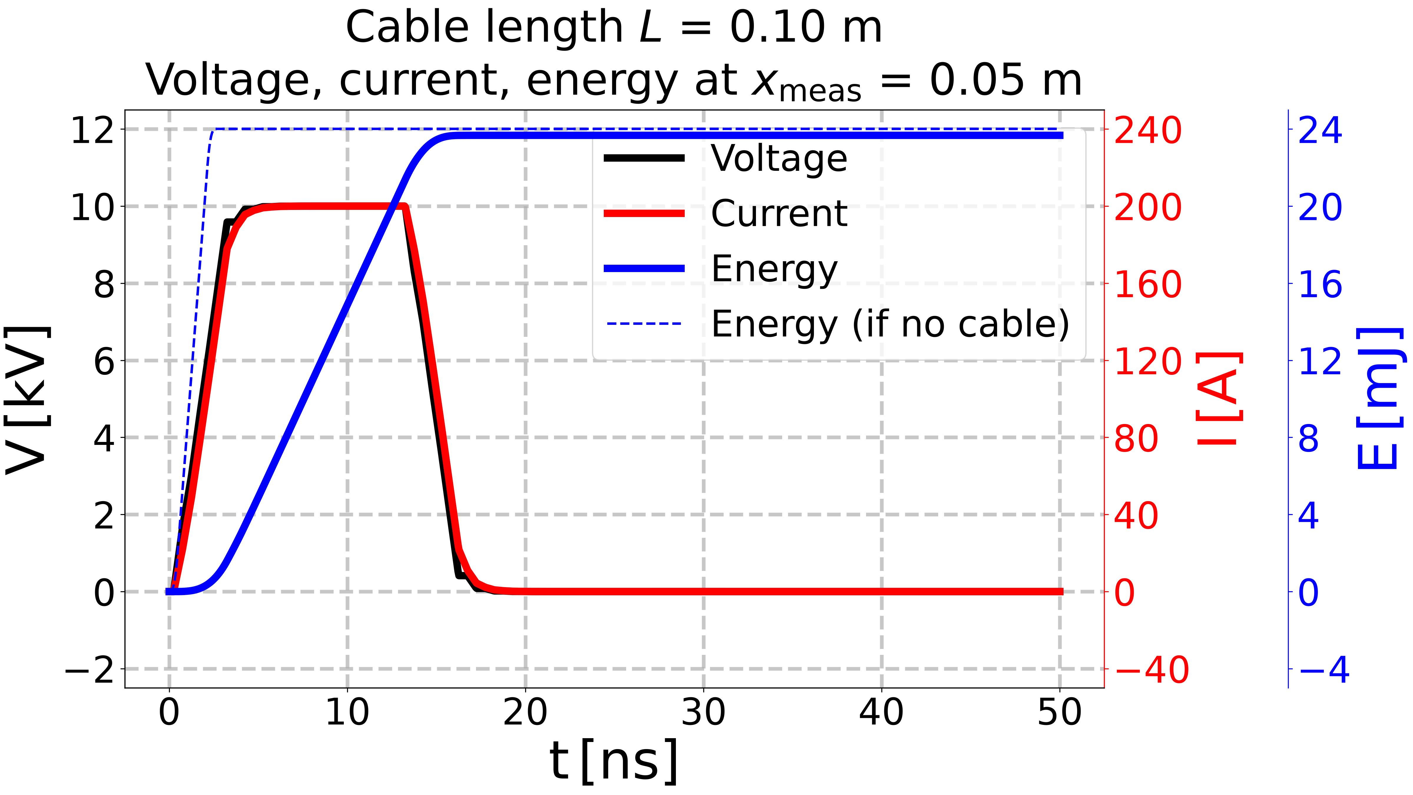
Cable length $L$ = 0.10 m
Voltage, current, energy at $x_{\mathrm{meas}}$ = 0.05 m
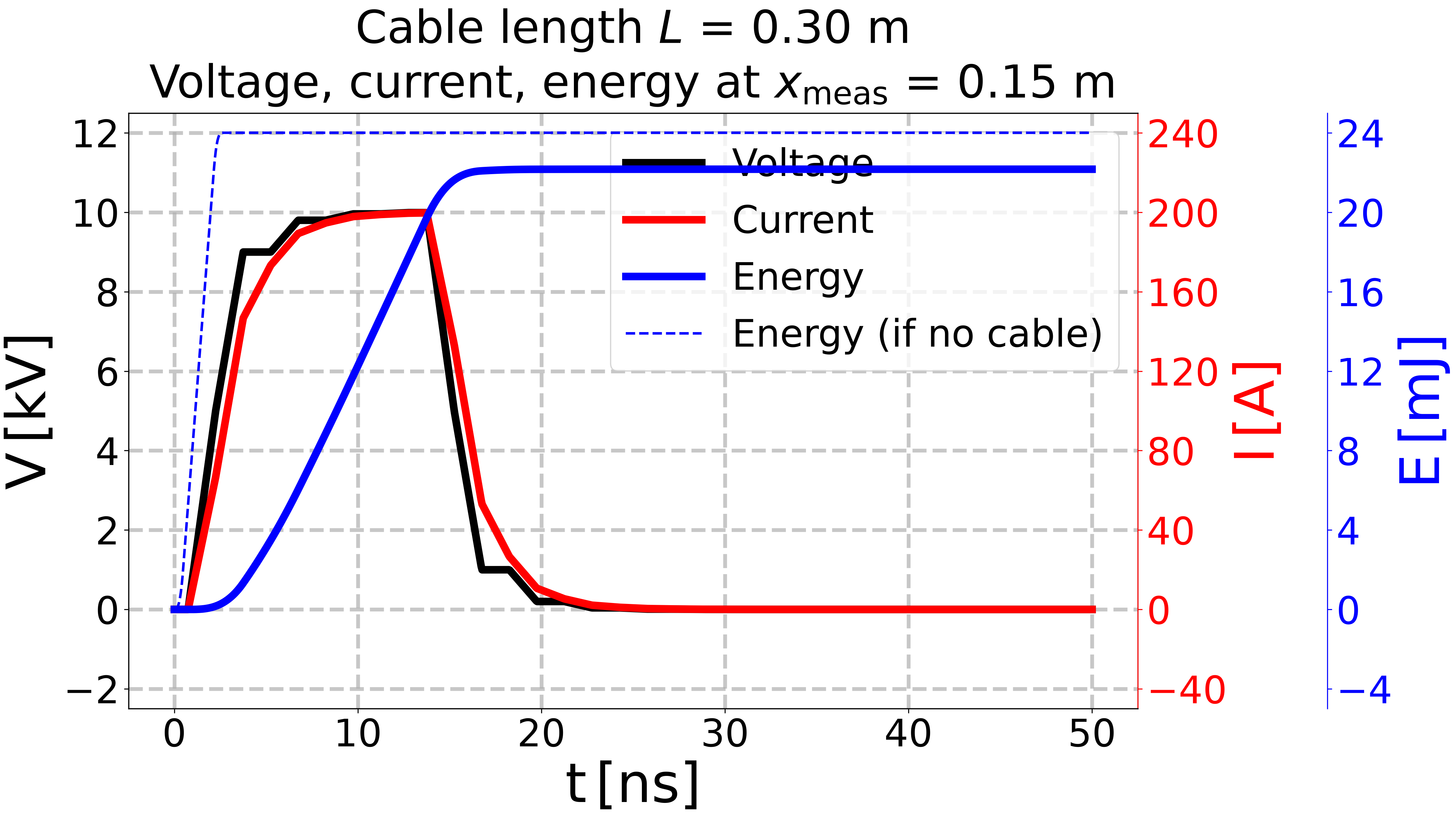
Cable length $L$ = 0.30 m
Voltage, current, energy at $x_{\mathrm{meas}}$ = 0.15 m
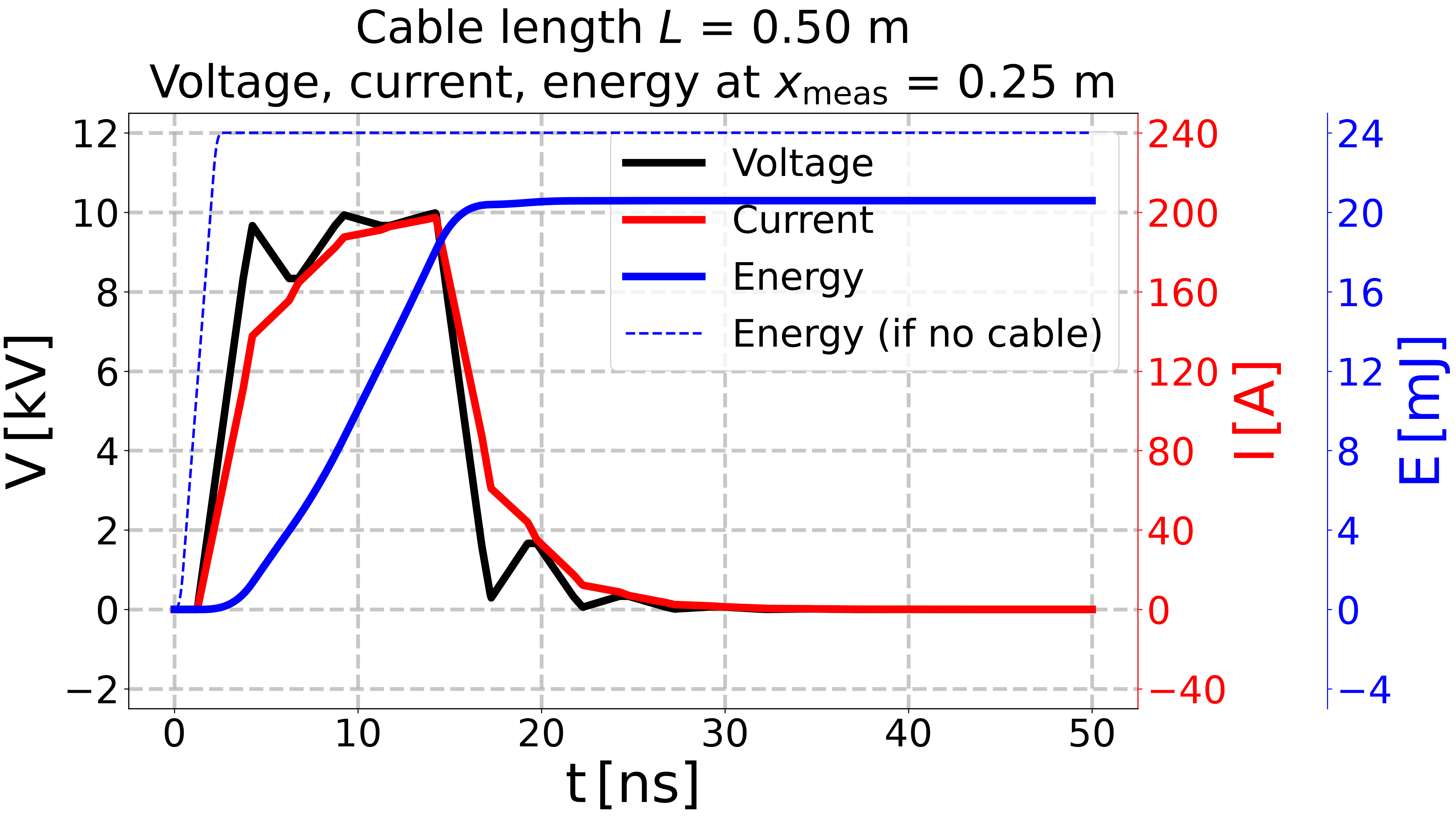
Cable length $L$ = 0.50 m
Voltage, current, energy at $x_{\mathrm{meas}}$ = 0.25 m
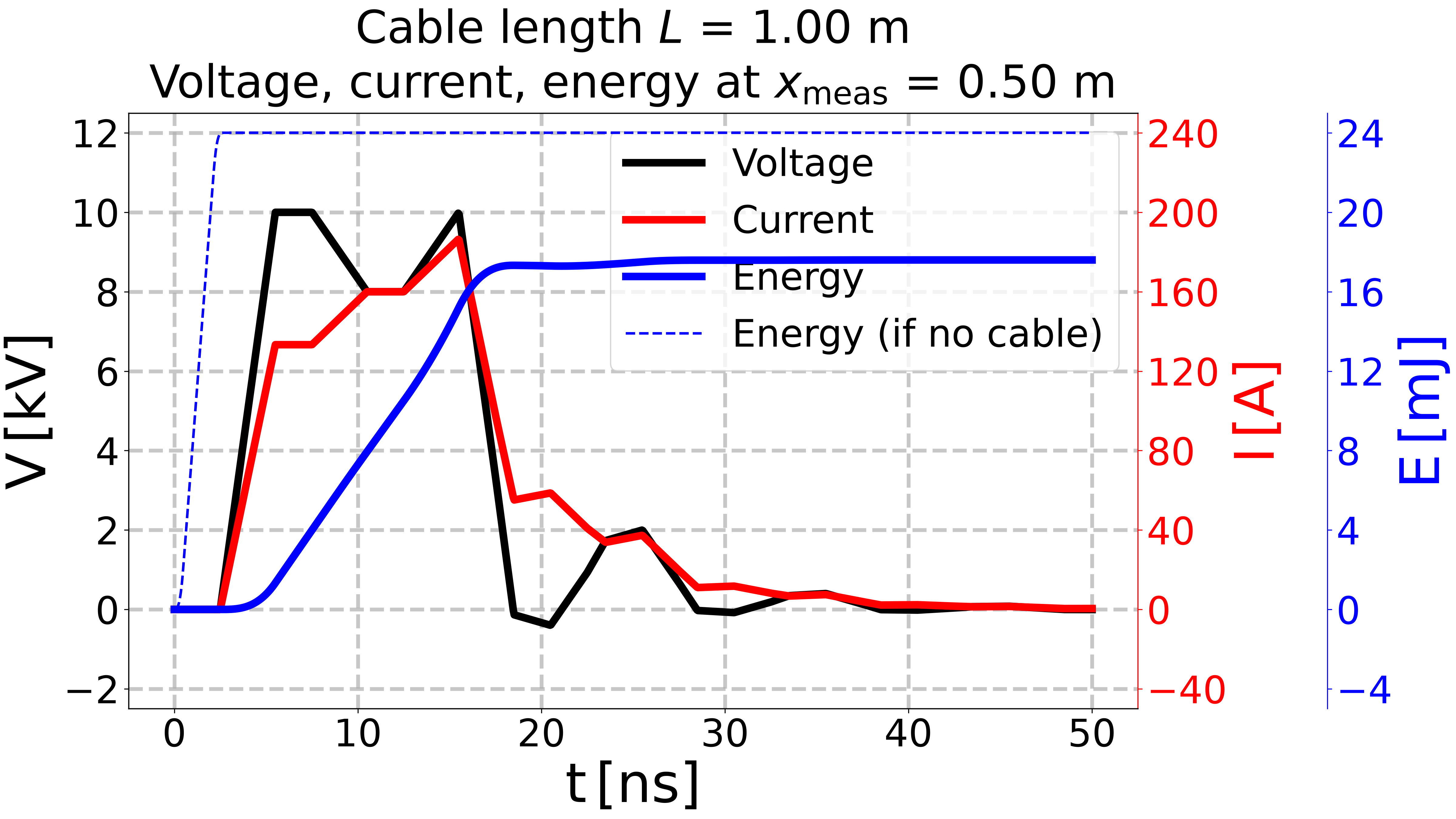
Cable length $L$ = 1.00 m
Voltage, current, energy at $x_{\mathrm{meas}}$ = 0.50 m
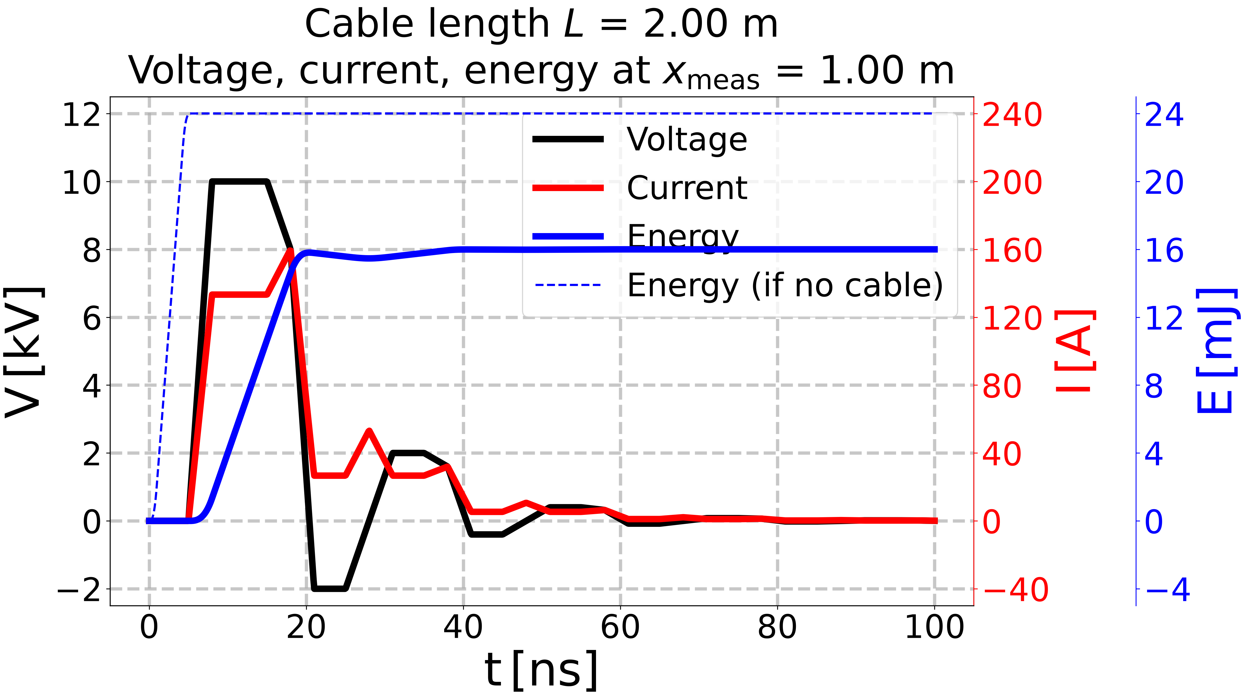
Cable length $L$ = 2.00 m
Voltage, current, energy at $x_{\mathrm{meas}}$ = 1.00 m
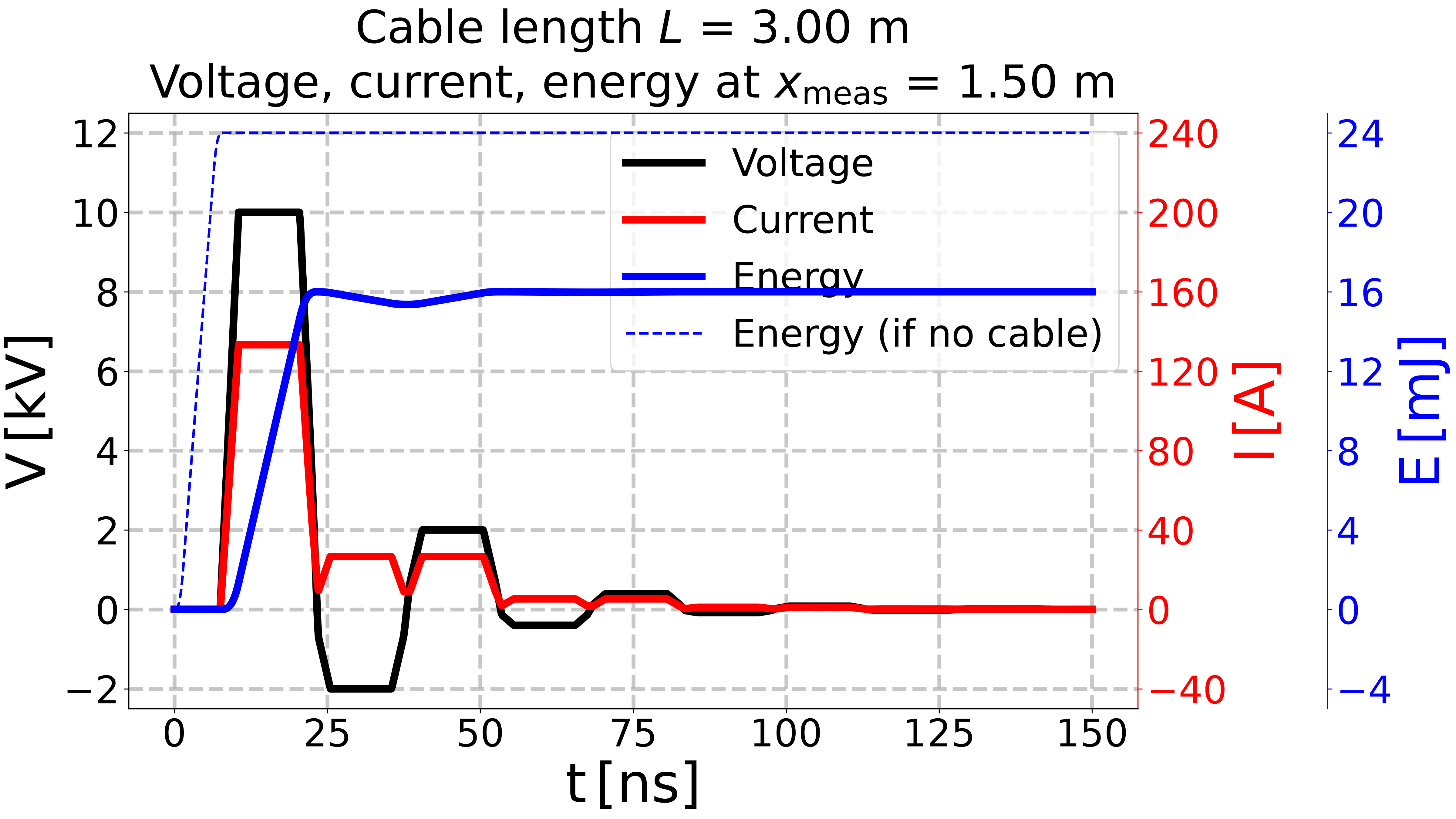
Cable length $L$ = 3.00 m
Voltage, current, energy at $x_{\mathrm{meas}}$ = 1.50 m
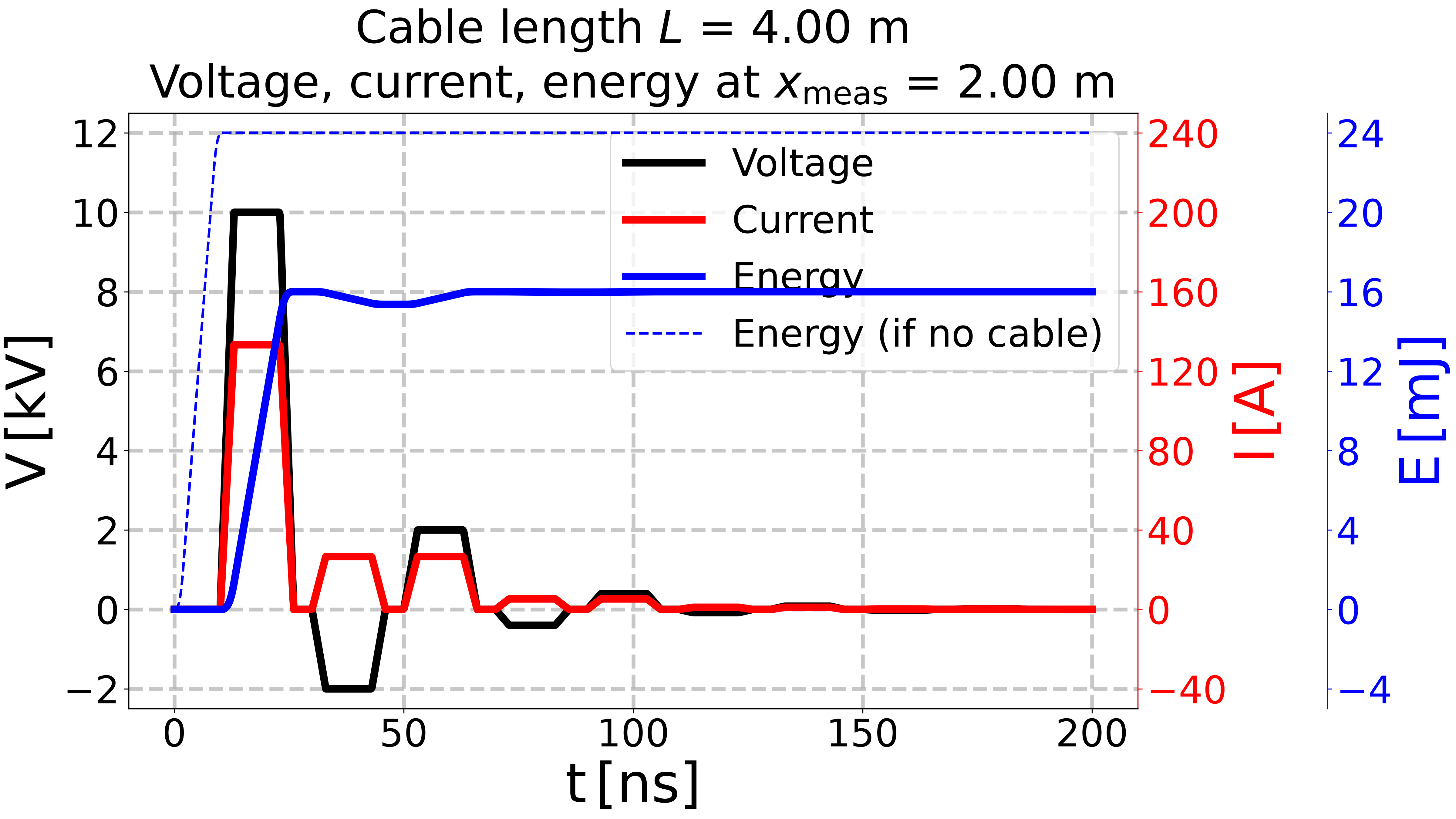
Cable length $L$ = 4.00 m
Voltage, current, energy at $x_{\mathrm{meas}}$ = 2.00 m
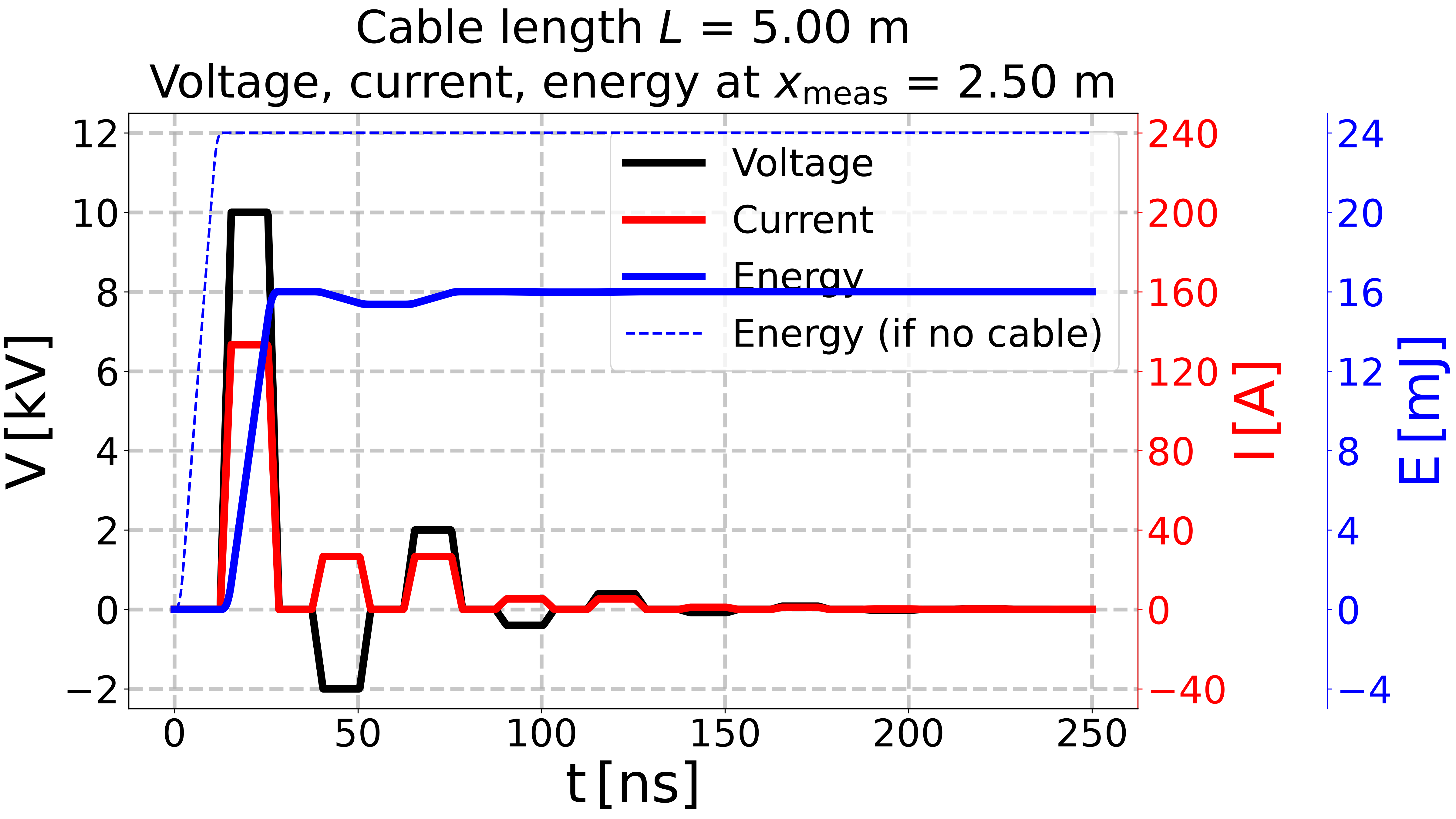
Cable length $L$ = 5.00 m
Voltage, current, energy at $x_{\mathrm{meas}}$ = 2.50 m
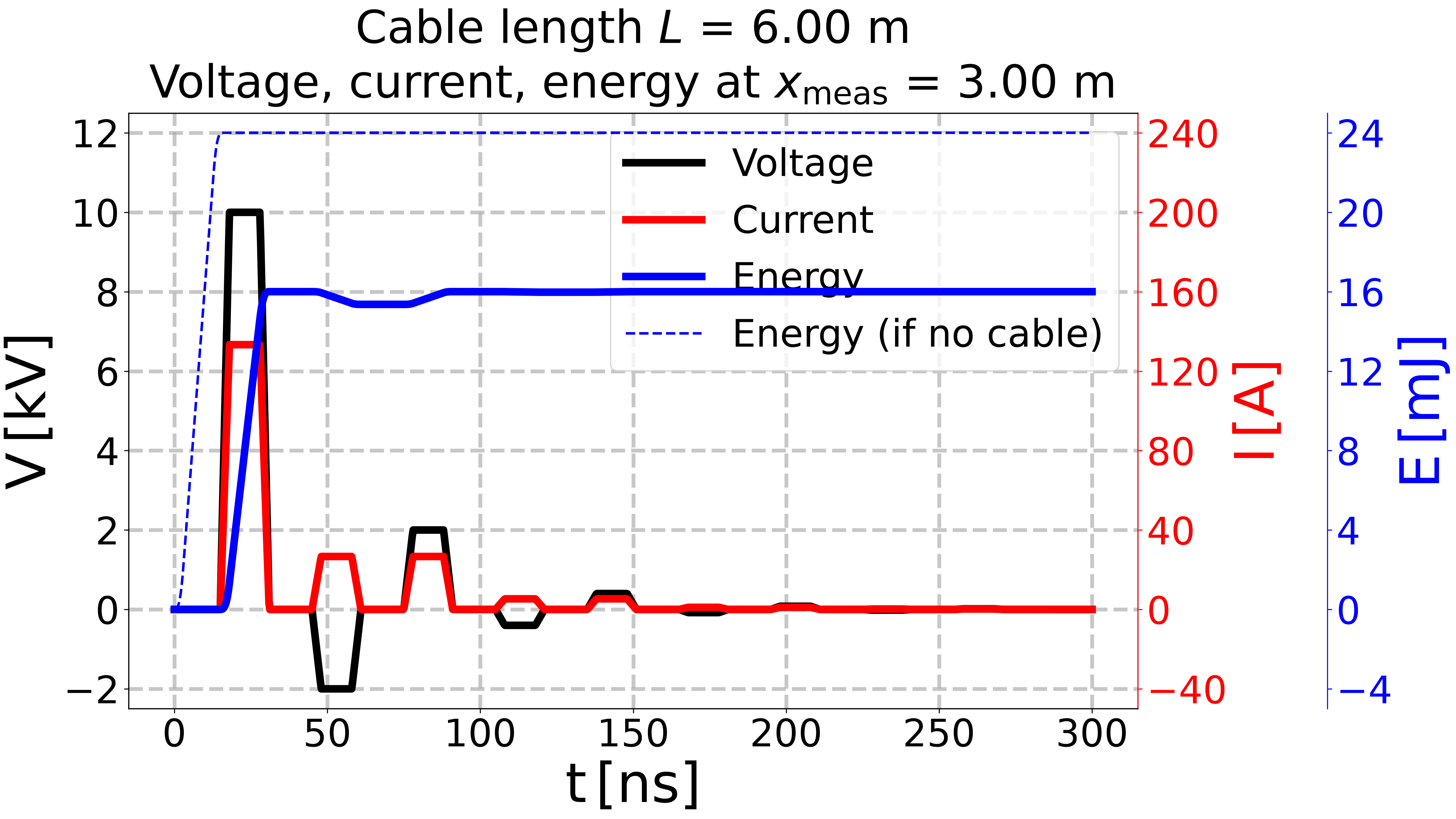
Cable length $L$ = 6.00 m
Voltage, current, energy at $x_{\mathrm{meas}}$ = 3.00 m